Surveillance Analysis Theory

A well-planned surveillance program is key to understanding reservoir performance and identifying opportunities to improve ultimate recovery. With surveillance analysis, you can perform Hall Plot and voidage replacement ratio (VRR) analyses. The Hall Plot analysis enables you to draw conclusions about average injectivity performance. The VRR analysis aids in identifying parts of a field where more or less water must be injected in order to reach or maintain VRR targets.

Hall Plot Analysis

The Hall Plot analyzes steady-state flow at an injection well. In general, the slope of Hall plot is interpreted as an indicator of the average well injectivity. At normal conditions, the plot is a straight line. Kinks on the plot indicate changes of injection conditions.

Hall (in 1963) presented this technique to interpret routinely collected injection well data to draw conclusions regarding near wellbore skin effects and average injectivity performance. The data required for Hall Plot analysis includes the following:

• monthly bottom-hole injection pressures (monthly average)
• average reservoir pressure
• monthly water injection volumes
• injection days for the month

The Hall method assumes steady-state injection such that the injection rate can be expressed as:

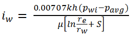(Equation 1)

where:

k = permeability,

h = reservoir thickness

pwi = flowing wellhead pressure

pavg = average reservoir pressure

μ = fluid viscosity

re = reservoir effective radius

rw = wellbore radius

S = skin

Equation 1 above is based on the following assumptions:

• the fluid is homogenous and incompressible
• the reservoir is vertically confined and uniform, both with respect to permeability and thickness
• the reservoir is horizontal and gravity does not affect flow (consequently, the flow is radial)
• flow is steady-state
• mobility ratio is equal to 1
• during the time of observation, the pressure at the distance equal to re is constant, and this distance itself is constant as well

At this point, it is assumed that k, h, μ, re, rw and S are constant. Therefore, Equation 1 reduces to:

(Equation  2)

where:

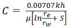(Equation 3)

Rearranging Equation  2 yields the following:

(Equation 4)

Integrating both sides of Equation  4 with respect to time gives:

(Equation 5)

The integral on the right hand side of Equation 5 is cumulative water injected. Hence Equation  5 can be represented as:

(Equation 6)

where:

Wi = cumulative volume of water injected at time t, bbls

Closer inspection of Equation 6 indicates that a coordinate graph of its left side of versus the right side should form a straight line with a slope of 1/C. This type of graph is called the Hall Plot. If h, μ, re, rw, and S are constant, then from Equation 3, the value of C is constant and the slope is constant. However, if the parameters change, C will also change and thus the slope of the Hall Plot will change, which is where the diagnostic value of the plot lies.

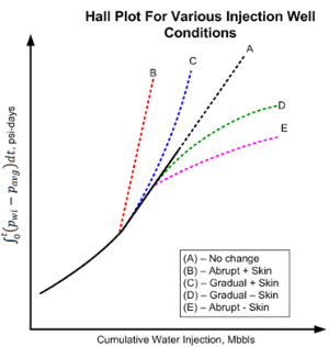
Changes in injection conditions may be noted from the Hall Plot. For example, if wellbore plugging or other restrictions to injection are gradually occurring, the net effect is a gradual increase in the skin factor, S. As S increases, C decreases; thus, the slope of the Hall Plot increases. Conversely, if S decreases (as would be the case if injecting pressure exceeds fracture pressure, causing fracture growth), then C increases and the slope of the Hall Plot decreases. See Figure 1 for various injection well conditions and their Hall Plot signatures.

Figure 1. Hall Plot characteristic signatures

The most challenging part of developing the Hall Plot is calculating the pressure-integral function of the y-axis. Fortunately, the integral can be easily solved. Consider Figure 2, which shows a graph of monthly bottomhole injection pressure, pwi, and periodic estimates of average reservoir pressure, pavg.

Figure 2. Bottomhole Injection and Reservoir Pressure vs. Time

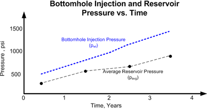
If it can be assumed that pwi and pavg are average for the month, then

(Equation 7)

where:

Δp = pwi - pavg

Δt = number of injection days for the month

Changes in the slope of the Hall Plot typically occur gradually, so several months (6 or more) of injection history may be needed to reach reliable conclusions about injection behaviour, as is the case for production decline curve analysis.

It is important to note that changes in the slope of the Hall Plot can be the result of other factors. Early in the life of an injection well (before gas fillup), the radius of the water and oil zones increase with cumulative injection and cause the value of C to increase, resulting in a concave upward trend in the Hall Plot. Recall that the Hall Plot technique assumes a mobility ratio of 1.0. If the mobility ratio is greater than 1, then the Hall Plot gradually trends concave downwards after gas fillup (as shown in curve D in Figure 1); if mobility ratio is less than 1.0, it will gradually trend concave upwards (see curve C). Also, as the average water saturation in the reservoir increases with time, kw may increase, which can also affect the slope of the plot.

If after gas fillup it can be assumed that pavg does not change significantly, then calculating the y-axis on the Hall Plot is greatly simplified by dropping pavg. This is because if pavg is constant and ignored, the Hall Plot is only shifted on the y-axis without changing the slope or its diagnostic interpretive value. Under this condition, the bottomhole injection pressure (pwi) is simply the wellhead injection pressure plus a hydrostatic gradient minus a frictional loss term. Since these two terms can usually be assumed to be constant and neglected, the left side of Equation 6 can simply reduce to the integral of the wellhead injection pressure, a dataset that is more readily available.

To determine whether average reservoir pressure is changing, it is necessary to conduct regular pressure buildup/falloff tests and to monitor monthly VRR plots. The objective of the Hall Plot is to detect changes in the injection well skin factor. It is not a perfect tool, but can, under certain conditions, provide reasonable insight on skin changes. The best tool for quantifying injection wellbore skin damage is a properly designed, well executed, and fully analyzed pressure fallout test.

References: Waterflooding Course, William M. Cobb & James T. Smith.

Voidage Replacement Ratio

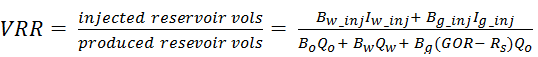
Voidage replacement refers to replacing the volume of oil, gas, and water produced from the reservoir by injected fluids. Voidage replacement ratio (VRR) is the ratio of reservoir barrels of injected fluid to reservoir barrels of produced fluid. Mathematically (for water and gas injection), VRR can be expressed as follows:

Equation 8

where:

Bx = formation volume factor for fluid type x

Ix = injected volume for fluid type x

Qx = produced volume for fluid type x

GOR = produced Gas Oil Ratio

Rs = solution Gas Oil Ratio

In Equation 8, the third term in the denominator accounts for free gas produced that is in excess of the gas in the reservoir that is dissolved in the oil.

VRR can be calculated on an instantaneous basis using injected and produced fluids over any specific time period (typically daily or monthly), with GORs calculated from instantaneous volumes. It can also be calculated on a cumulative basis using cumulative injected and produced fluids, with GORs calculated from cumulative fluids. In the latter case, it is common to start the cumulative production numbers at the start of injection. But in some cases, there is value in starting the cumulative production numbers at the start of production. Figure 3 shows Instantaneous VRR and Cumulative VRR datasets for a sample set of wells.

Figure 3. Instantaneous VRR and Cumulative VRR datasets for a sample set of wells

Due to leaking faults, poor cement casing bond, discontinuous sands depleted prior to water injection, a gas cap, or an inactive aquifer, it is common to lose some of the injected water to areas outside of the floodable pore volume.

If the Instantaneous VRR for a given month is equal to or greater than 1.0, the reservoir pressure is being maintained or increased for the month. If the ratio is less than 1.0, reservoir pressure declines for the month. When computing the reservoir voidage, it should not be assumed that the free gas term is negligible without making appropriate calculations.

As long as cumulative VRR is equal to or greater than 1.0, after taking into account injection losses, reservoir pressure since the start of water injection will be maintained or increased. When the cumulative VRR calculated since the start of production reaches 1.0, reservoir pressure will have increased to near original reservoir pressure (pi).