Compound Linear Typecurve Analysis

Compound linear typecurves are useful for analyzing horizontal multifrac wells producing from tight gas or shale wells.

Note: For more information on Compound Linear typecurve theory and equations, see Compound Linear Typecurve Theory.

This method uses the horizontal multifrac model.

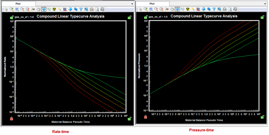
There are two sets of compound linear typecurves:

1. Pressure-time: uses normalized pressures - the constant rate solution

2. Rate-time: uses normalized rates - the reciprocal of the constant rate solution

Rate-time and pressure-time are reciprocals of one another, and simply plot the data on the typecurves differently.

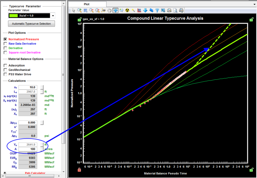
Boundary-Dominated Match

As the compound linear typecurves were developed using an infinitely large reservoir, there is no boundary-dominated flow stem. However, entering a value for either Ye or Area (A), will produce a dashed boundary-dominated flow line that intersects the selected typecurve.

Note: A typecurve must be selected before the boundary-dominated line is plotted.

If boundaries have been reached, the production data will deviate from the compound linear typecurve onto the boundary-dominated line.

Transient Match

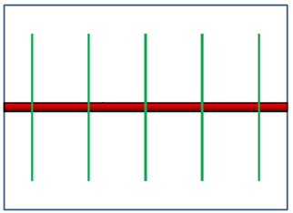
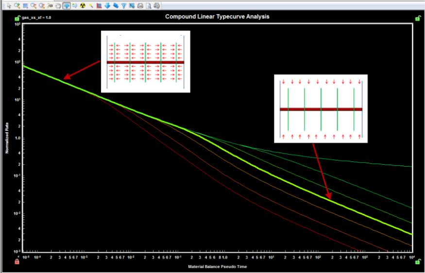
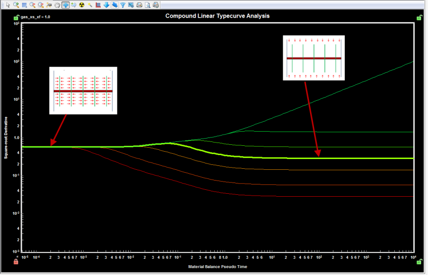
Compound linear typecurves were developed for a horizontal, multifrac well in an infinite reservoir. The first half slope indicates linear flow into the fractures, while the second half slope indicates linear flow into the fractured region. The two half slopes are connected by a transition period. Most production data is expected to fall in the transition zone.

Selecting the "Square Root Derivative" plot will display the linear flow periods as flat lines, which may be helpful for matching data.

Matching data to a typecurve will give the Xs / xf ratio. Entering a value for number of fractures (n_f) will calculate the following values:

Le
xfsqrt(k)
Xs sqrt(k)
(xf)y
Xs

Note: Entering a value for Le will calculate n_f.

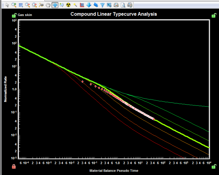
Skin

Generally, skin effects will impact the first linear flow period, causing the data to deviate from the ideal typecurve.

To correct for skin effects on the Normalized Pressure or Rate curves:

1. Match the later part of the data to a typecurve.

2. Select the typecurve that matches the data most closely.

3. Enter the number of fractures (n_f) or Le.

4. Right-click the plot and hold your mouse button. This will highlight the data point closest to the top left corner for Rate-Time (bottom left for Pressure-Time), and the cursor will change to a triangle.

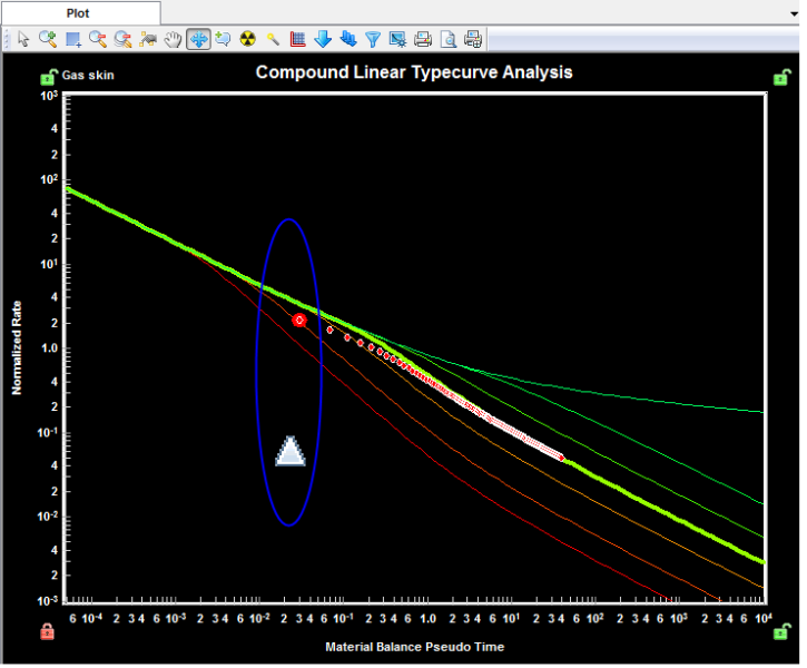
5. While continuing to hold the right-mouse button, move the cursor up or down until the early portion is matched on the typecurve.

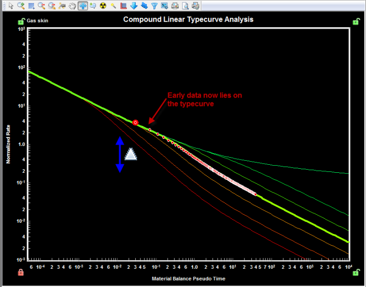
Moving the data in this manner will populate the cell. This value is then used to convert the dimensionless pressure drop into an equivalent apparent skin, apparent fracture conductivity, and dimensional pressure drop.

For more details on the calculations, see Compound Linear Typecurve Theory.