Fetkovich Typecurve Analysis
The Fetkovich typecurve analysis (SPE 004629, 1980) was the first analysis method to use analytical typecurve matching for production data. It is a semi-analytical approach in that typecurves are generated from analytical solutions of transient (infinite) radial systems at constant flowing pressure, while the boundary-dominated flow period is defined using hyperbolic decline typecurves, originally developed by Arps. In addition to reserves, calculated from the depletion stem (b-value) match, this analysis provides diagnostic power through the determination of reservoir permeability and wellbore skin factor. Rate normalization (SPE 012179, 1984) has been included to account for changing operating conditions (i.e., changes in flowing pressures) to more reliably determine permeability and skin. With re-initialization, you can analyze the transient production data signature of post-buildup production to diagnose permeability and skin. A clear advantage of this method over modern typecurve methods is that it does not plot data using superposition time functions, which may bias the interpretation. It remains a popular technique for the analysis of conventional vertical oil and gas wells. Fetkovich plots are even used to describe the behaviour of unconventional well production data (e.g., Bakken oil wells). The limitation of this technique is that the transient typecurves are restricted to radial flow systems, and the method does not directly calculate original-hydrocarbons-in-place (as is the case in modern methods); it is estimated through simple material balance.
Note: For information on the Fetkovich typecurve theory and equations, see Fetkovich Typecurve Analysis Theory.
The Fetkovich typecurve analysis method uses the following models:
- Radial
- Fracture (rectangular)
Boundary-Dominated Match
To obtain information about reserves and drainage areas, we recommend that you focus on the boundary-dominated (depletion) stems of the typecurves. These are located to the right of where the Rate vs. Time and the Cumulative Production vs. Time typecurves intersect. Each of the depletion stems represents a different b value, identical to the b values used in the hyperbolic Arps analysis. Once a b value has been selected, Harmony calculates recoverable reserves and expected ultimate recovery. If a sandface flowing pressure is specified on the Analysis tab, Harmony also calculates drainage area and original gas-in-place.
Transient Match
To obtain information about permeability and skin, we recommend that you focus on the transient stems of the typecurves. These are located to the left of where the Rate vs. Time and the Cumulative Production vs. Time typecurves intersect. Each of the transient stems represents a different reD value. Once a reD value has been selected and a sandface flowing pressure is specified, Harmony calculates permeability and skin.
Time Reinitialization
The fundamental assumption in Fetkovich transient analysis is a constant sandface flowing pressure. Although an ideal case, this assumption is rarely representative of true operating conditions, particularly in early (transient) production. A well may be subject to shut-ins or operational changes during its life. When a well is shut-in or undergoes a change in operating conditions, the constant sandface flowing pressure assumption is no longer valid. When the well resumes production, a new additional transient effect is introduced to the wellbore. Additional transient effects in the wellbore are indicated by the green arrows in the screenshot below.
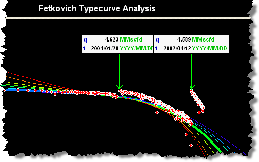
Fetkovich suggested a method called "time reinitialization" to analyze a dataset with multiple transient effects. This method resets the time at the start of each additional transient effect to zero, allowing you to specify additional transient effects on the typecurve plot. Once specified, the time associated with the first rate of each new transient flow period is reset to zero. As a result, the dataset is smoothed on the typecurve, allowing you to continue with the Fetkovich typecurve match.
To perform a Fetkovich time reinitialization:
1. Identify the beginning of each additional transient flow period either from Fetkovich or the Raw Data plot.
2. Click
the Add Reinitialization Arrow
icon (![]() )
on the Fetkovich plot tool bar.
)
on the Fetkovich plot tool bar.
3. Click the data point representing the beginning of the additional transient flow period. The green reinitialization arrow is displayed at that point.
![]()
- Move the arrow left and right using the arrow keys on the keyboard.
- Remove the arrow by clicking the arrow's annotation box, and then pressing the Delete button on the keyboard.
Note: To create multiple additional transient periods, click the Add Reinitialization Arrow icon again, then repeat the process explained above. (The maximum number of additional transient periods permitted in Harmony is ten.)
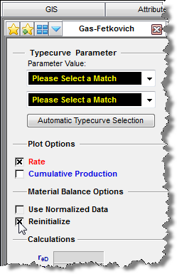
4. Select the Reinitialize option under Material Balance Options in the parameters pane.
5. Continue with the Fetkovich typecurve matching analysis method.