Analytical Models Analysis Theory

Modeling is the process of history matching pressure and rate transient data based on a mathematical model. There are many different models available to match the data depending on the situation. Thus, it is important to analyze the pressure and rate transient data before modeling because it forces the analyst to think about the probable reservoir configurations and provide good estimates of reservoir parameters. Models are not unique (different model types can match the same set of data), and as a result, we recommend selecting the model type after the analysis step. The following summarizes the advantages of modeling pressure and rate transient data:

• Modeling makes use of all the information within a dataset. For example, while analyzing data from vertical wells, the analyst might try and determine permeability and skin by analyzing the data points that make up the zero slope on the derivative plot, and the semi-log straight line on the radial plot, but ignore the data points in the transition period between wellbore storage and radial flow. Models make use of the information contained in transition periods.
• Modeling takes all flow regimes into account. In multi-rate situations, analyses depend on the superposition of the equation for a single flow regime. For example, the derivation of Horner time includes the assumption that all flow, including the entire drawdown, is radial. Modeling doesn’t assume that only one flow regime has occurred.
• With modeling, you can simultaneously analyze multiple flow periods, so that a single set of parameters can be found.

Parameter values obtained during the analysis step provide a good starting point for an appropriately chosen model type. Parameters can then be optimized by automatic parameter estimation (APE). Before using the APE method, corrupted data should be removed from the dataset to prevent the attempt to match of invalid points.

Choice of Model

As stated above, different models can be used to match a single set of data. Choosing a probable model type requires the consideration of a number of factors including seismic data, geology, log data, and information provided from other wells drilled in the same formation.

The choice of model can drastically change the outcome of a forecast. For example, pressure and rate transient analysis of radial flow data can be used to find the reservoir flow capacity (kh). If heterogeneity is observed in the data, one might use the composite model with different values for permeability in each zone. Another analyst might decide that using a two-layered multilayer model, having different net pays, is more probable. The forecast of the composite and multilayered models for this situation can differ drastically, even though both models can match the test data. The analyst must decide which model is better.

Model Assumptions

There are many assumptions that go into the model itself which can lead or mislead the analyst. Most models assume that a reservoir is homogeneous (dual porosity excluded, where the dual porosity flow within each layer can be modeled either as pseudo-steady state or transient interporosity flow). There is no single reservoir that is actually homogeneous in nature, but many reservoirs behave as homogeneous reservoirs.

For example, the composite model assumes that reservoir properties change at a certain radius from the reservoir. This phenomenon also doesn’t necessarily occur in nature, yet some reservoirs behave as though they are composite reservoirs. An example of this is an injection well, where the fluid properties (compressibility and viscosity) change at a certain distance from the wellbore. The composite model can be used to match many data sets, so it is important that it is not overused. However, there are cases where it is the appropriate model to use.

Vertical Model

The vertical model simulates the pressure response in a vertical well within a rectangular-shaped reservoir with homogeneous or dual-porosity characteristics. Note that the well may be at any location within the reservoir, and that the reservoir for the vertical model has no-flow boundaries. During very early times, the cylindrical source solution is used, which is followed by the Green’s function solutions (Gringarten and Ramey, 1973). No-flow boundaries are modeled using the method of images. The result is superposed in time based on the rate history provided.

Fracture Model

The fracture model simulates the pressure response in a vertical well intercepted by an infinite-conductivity vertical fracture within a rectangular-shaped reservoir with homogeneous or dual-porosity characteristics (see the figure below). Note that the well may be at any location within the reservoir, and that the reservoir for the fracture model has no-flow boundaries. During very early times, the cylindrical source solution is used, which is followed by Green’s function solutions. The Green’s function solution, as developed by Thompson et al. (1991), is used with slight modifications to simulate an infinite-conductivity vertical fracture. No-flow boundaries are modeled using the method of images. The result is superposed in time based on the rate history provided.

Horizontal Model

The horizontal model simulates the pressure response in a horizontal well within a rectangular-shaped reservoir with anisotropic heterogeneities (i.e., differences in permeability in the x, y, and z directions), or dual-porosity characteristics. The anisotropy is handled using a conformal mapping procedure that adjusts the boundary sizes accordingly to mimic the effect of increased or decreased permeability in each direction. The horizontal well is oriented in the x-direction and may be at any location within the reservoir (see the figure below) and supports no-flow boundaries.

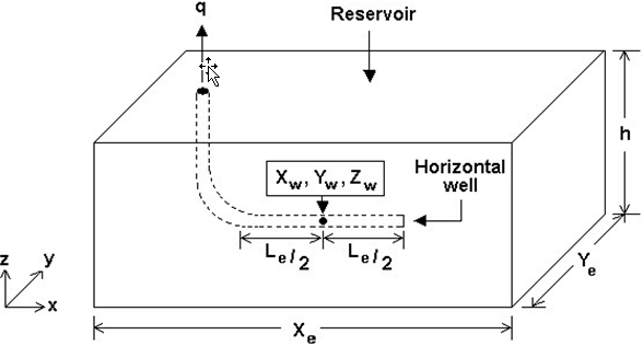
Note that the effective wellbore length (L_e) defines the wellbore area open to fluid flow. The cylindrical source solution is used at very early times, which is followed by Green’s function solutions for horizontal wells, as developed by Thompson et al. (1991). No-flow boundaries are modeled using the method of images. The result is superposed in time based on the rate history provided. The following flow regimes can be handled by this model:

• Wellbore storage
• Vertical radial flow
• Linear horizontal flow
• Elliptical flow
• Horizontal radial flow
• Boundary effects
• Pseudo-steady state flow

Multilayer Model

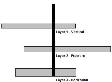
This model simulates the commingled flow from any number of independent layers as shown below. Each layer can have its own model type (e.g., vertical, fracture, horizontal, etc.). All layers are considered to have an identical initial pressure (p_i), but other parameters (i.e. skin, permeability, net pay, etc.) can be set independently in each layer. No crossflow between the layers can occur, except at the wellbore.

Composite Model

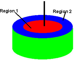
Composite models are used when reservoir (e.g. permeability, net pay, and total porosity) and fluid (e.g. compressibility and viscosity) properties change at some distance from the wellbore. The figure below shows an example of a two-zone (region) composite reservoir.

With the composite model, you can add any number of different cylindrical zones. With an unlimited number of zones, virtually any pressure or rate transient response could be matched. Therefore, it is important to exercise good judgment to determine when this model is appropriate. No reservoir is perfectly cylindrically concentric composite in nature; however, many reservoirs do behave the same way as composite reservoirs do. Some common situations where the composite model is useful include injection cases (which cause changes in viscosity and compressibility), reservoir heterogeneities (such as changes in flow capacity (kh)), and cases where the well was drilled into a naturally fractured reservoir with varying fracture distribution.

Note that the following assumptions apply when using this model:

• Both the inner and outer regions can be assumed to be homogeneous or dual porosity
• The wellbore has a finite volume and an infinitesimal skin
• There is no transition region between the inner and outer regions

Water-drive Model

The water-drive model is a cylindrical reservoir with concentrically cylindrical aquifer. The outer zone represents the aquifer and can have any radius (provided that it is larger than the reservoir radius).

The water-drive model is an analytical radial composite reservoir model. The reservoir is represented by the inner zone, and is given a radius of "re". The outer zone represents the aquifer, with a radius of "raq". The aquifer radius may be set to any value greater than "re". The model accounts for the mobility difference between reservoir and aquifer by enabling you to enter a mobility ratio (M). This is defined as the ratio of the aquifer mobility to that of the reservoir.

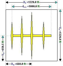
Horizontal Multifrac Composite Model

The horizontal multifrac composite model is a rectangular model that contains a non-contributing horizontal well fed by multiple identical and equally-spaced transverse fractures. The portion of the reservoir between the fracture tips and the entire reservoir length is defined as the inner reservoir and the rest is the outer reservoir, as illustrated in the figure below. The permeabilities of the inner and outer regions can differ, making this model useful for modeling a stimulated reservoir volume (SRV) created by hydraulic fracturing, which is fed by an unstimulated outer region.

This model calculates the reservoir's response from early-time storage and fracture flow, through the transition into boundary-dominated flow. The fundamental building block of this model is the tri-linear fracture model for a vertical well. The outer reservoir feeds the inner reservoir via linear flow. The inner reservoir feeds the fractures via linear flow, and the fluid within the fractures travels linearly towards the wellbore. However, for a horizontal well, the fluid within transverse vertical fractures actually has a radial flow pattern, and a convergence skin has been implemented in order to account for this. As a result, it is not possible to observe radial flow with this model.

Note:   A detailed description of the model is given by Brown et al. (2009).

You can specify the reservoir dimensions, number of fractures and fracture half-length, provided that the entire wellbore and all fractures fit within the reservoir boundaries. The dimensionless fracture conductivity must also be specified. Dual-porosity behaviour can be modeled within the inner reservoir, but the outer reservoir remains strictly homogeneous. A turbulence factor (D) can also be specified.

Horizontal Multifrac SRV (Uniform Fracs) Model

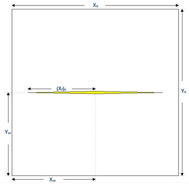
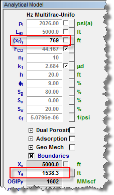
This model is the same as the horizontal multifrac composite model, but includes only the inner region of the reservoir — not the outer reservoir region. In this model, fracture tips always extend to the edge of the reservoir.

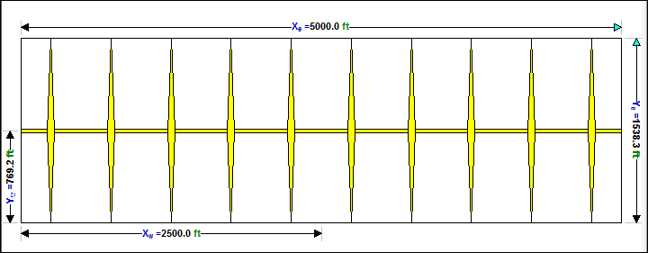
In this model, (xf)y is always half of Ye. Changing the value of one dynamically changes the value of the other.

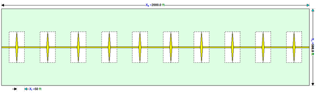
Horizontal Multifrac Enhanced Fracture Region Model

This model is a rectangular reservoir model consisting of a non-contributing horizontal well and transverse fractures. This model assumes that all the fractures are uniformly spaced with equal half-fracture length. (The reservoir can extend beyond the fracture tips.) This model has an improved effective permeability region around each fracture, and you can specify the distance from the fracture to the permeability boundary (X_I).

This model takes the following linear flow regimes into account:

• linear flow within the fracture (at very early time)
• linear flow within the stimulated region towards the fractures
• linear flow within the non-stimulated regions towards the stimulated region
• linear flow within the non-stimulated region towards the wellbore

Note:   A detailed description of the model is given by Stalgorova and Mattar (2012).

General Horizontal Multifrac Model

The general horizontal multifrac model is a homogeneous, single-phase, rectangular reservoir model consisting of a horizontal wellbore and transverse fractures. The horizontal multifrac solution is created through the superposition of individual infinite conductivity fracture solutions in space.

You can specify the reservoir dimensions and well position, provided the entire wellbore and all fractures fit within the reservoir boundaries. In addition, each fracture can be situated anywhere along the horizontal wellbore and configured to have a unique fracture half-length and conductivity. Thus, it is possible to model the combined effects of the horizontal wellbore and multiple fractures, as well as the transition into middle-time flow regimes and boundary-dominated flow for any number of different geometrical configurations. Depending on the configuration, pseudo-radial flow can be observed with this model.

Damage skin is applied along the length of the horizontal wellbore and a turbulence factor may be specified.

Horizontal Multifrac Repeating Pattern Model

The multifrac repeating pattern model is a homogeneous, single-phase, rectangular reservoir model consisting of a horizontal wellbore and transverse fractures. The wellbore is located in the center of the reservoir. Fractures are considered to be symmetrically distributed within each stage and all stages are identical.

Because all fractures follow a repeating pattern, after you specify fracture locations, fracture half-lengths, and fracture conductivities for one stage, the parameters of the rest of the stages are populated automatically.

Prior to calculating the entire system’s solution, the model generates the solution for one single stage through superposition of individual infinite conductivity fracture solutions in space. Then, the entire system’s solution is calculated by multiplying the single stage’s solution by the number of stages. Consequently, the speed of calculation is improved, and depends on the number of fractures in each stage, rather than the total number of fractures.

This model is similar to the general horizontal multifrac model, and it can model the combined effects of the horizontal wellbore and multiple transverse fractures, as well as the transition period between flow regimes. Skin is applied along the length of the horizontal wellbore and a turbulence factor may be specified.