Beta-Derivative Theory

The β-derivative is a diagnostic tool for identifying power-law type flow regimes (such as wellbore storage, linear flow, bilinear flow, boundary-dominated flow, etc). It was proposed for the analysis and interpretation of pressure transient data by Hosseinpour-Zonoozi et al. (2006) and was later modified by Ilk et al. (2007) as a rate-based function to analyze production data for the purpose of estimating reservoir properties and contacted in-place fluid. Power-law type flow includes those transport regimes whose solutions are of the form:

Equation 1

where:

n = 1 for wellbore storage and boundary-dominated flow

n = ½ for linear flow

n = ¼ for bilinear flow

n = -½ for spherical flow

A and B are dependent on the properties of the fluid-rock system in question. It is obvious from this definition that radial flow does not fall into this category of flow regimes.

The definition of the β-derivative for constant rate and constant pressure production are given respectively as:

Equation 2: Constant Rate

Equation 3: Constant Flowing Pressure

The β-derivative is unitless. It possesses a unique character for different flow regimes. For instance, it is 0.5 for linear flow, 0.25 for bilinear flow and 1.0 for both boundary-dominated flow and wellbore storage. Since radial flow is not a power-law type of flow regime, it does not yield a constant β-derivative.

Beta-Derivative for Constant Rate and Constant Pressure Production

Constant rate and constant pressure production are well understood flow scenarios whose solutions are available in the literature. In dimensionless form, their β-derivative is given by:

Equation 4

Equation 5

where

For example, the β-derivative plots (on a log-log scale) for constant-rate and constant-pressure production from an infinite conductivity fracture in a bounded reservoir are as shown in the figure below.

Figure 1: Beta-derivative plot for constant rate and constant pressure production

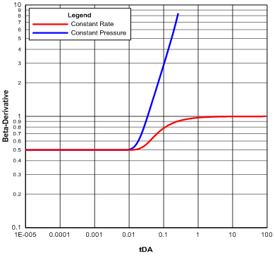
In the transient linear flow regime, the derivative is 0.5 for both production scenarios. However, the derivatives separate in the boundary-dominated flow regime—the β-derivative for the constant rate production approaches 1 in the late time, taking on a characteristic “S” shape, while that for the constant pressure production assumes a unit slope straight line trend.

Equivalence of Constant Rate and Constant Pressure Production

Palacio and Blasingame (1999) and Anderson and Mattar (2003) have demonstrated that under boundary-dominated flow, constant-pressure production can be converted into its equivalent constant-rate production using a superposition function called the material-balance time. Mathematically, the material-balance time is given by:

Equation 6

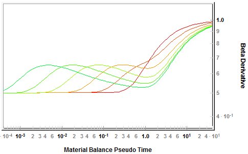
where QDA is the dimensionless cumulative production given by . When the material-balance time is used, the β-derivative plots for the constant-rate production and the constant-pressure production become identical, for all practical purposes. Figure 1, when recast in terms of material-balance time, is as shown in Figure 2.

Figure 2: Beta-derivative plot referenced to material-balance time

Beta-Derivative for Variable Rate and Variable Pressure Production

Under actual conditions, it is difficult, if not impossible, to constrain field production to constant rate or constant bottomhole flowing pressure—both rate and wellbore pressure often vary. To conveniently analyze field production data, it is therefore necessary to transform actual production conditions into an equivalent ideal condition whose solution and analysis methods are well developed. In this regard, the material-balance time function is used to convert variable rate/variable pressure production into an equivalent constant rate production.

The β-derivative, in this case, is defined in terms of normalized quantities (rate or pressure) as:

Equation 7

Note:   Note the negative sign in Equation (7).

Equation 8

where:

tc = Np / q is the material-balance time.

If the produced fluid is gas, pseudo-pressure, ∆pp, and material-balance pseudo-time, tca are used (in place of pressure and material-balance time) to render gas production analyzable using the techniques designed for liquid production. Using either Equation (7) or (8) for the analysis of variable rate/variable pressure production data is a matter of choice, as there is no substantive difference between both approaches.

Actual field production data is inherently noisy and of low frequency compared to welltest data. The noise is further amplified in any diagnostic analysis that involves computing the derivative of the data, thereby making it difficult, if not impossible, to identify the trends sought after in the resulting data plots. Such is the case with the β-derivative obtained from noisy production data. It is therefore advantageous to de-noise (i.e. smooth) the data. Blasingame et. al (1989) introduced a method of smoothing noisy data by using integration. The smooth, auxiliary function obtained from integrating normalized rate through time is called the normalized rate integral (rate integral, for short).  In concept, rate integral is the average normalized rate at which a well has produced until a particular time, and is defined as:

Equation 9

For practical purposes, the β-derivative is formulated in terms of the rate integral. Ilk et al. (2007) called this formulation the β-integral derivative.

Equation 10

Recognizing that d(lny) / d(lnx) = 1/y * dy / d(lnx), Equation 10 can be rewritten as:

Equation 11

The denominator of Equation 11 is the rate integral while the numerator is the rate-integral derivative (i.e. the semi-log derivative of the rate integral). This means that the β-integral derivative can simply be calculated as:

Equation 12

In terms of the pressure integral, the β-integral derivative is calculated thus:

Equation 13

Given a set of production data, Figure 3 compares the β-derivative plots generated using both Equations 12 and 13.

Figure 3: Comparing the two different β-integral derivative formulations

Both plots convey the same message—transient linear flow followed by boundary-dominated flow—although the Normalized Pressure Integral formulation is more distinctive at the start of boundary-dominated flow. The remaining part of this document will focus on the Normalized Rate Integral approach.

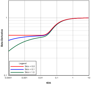
Effect of Skin on the Beta-Derivative

Actual production is oftentimes affected by non-ideal conditions near the wellbore, which manifest as an extra pressure drop at the sandface. In modeling, this extra pressure is treated as a skin effect. Figure 4 shows the β-derivative plot for a skin-free constant rate production alongside two other plots for the same production scenario but with skin effects present. It is observed that the classic 'S' signature of the beta-derivative is distorted in the presence of skin. Therefore, skin masks the sought-after signal in a β-derivative plot.

Figure 4: Effect of skin on the beta-derivative

Beta-Derivative Typecurves

Figure 5: β-Derivative Typecurves for Blasingame Fracture Model

Figure 6: β-Derivative Typecurves for Agarwal-Gardner Fracture Model

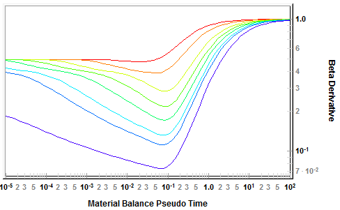
Figure 7: β-Derivative Typecurves for NPI Fracture Model

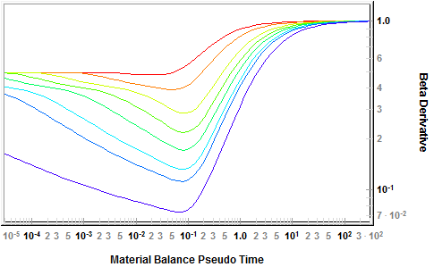
Figure 8: β-Derivative Typecurves for Wattenbarger Fracture Model

The β-derivative is a ratio function. Its dimensional (data) and dimensionless (typecurve) formulations are the same. When both formulations are plotted on the same graph, they are automatically aligned on the vertical scale—only a horizontal shift of the data plot is needed to obtain a typecurve match. Therefore, when used in conjunction with existing typecurves, the β-derivative helps reduce the uncertainty and non-uniqueness problems often encountered in typecurve matching.

Data Preparation

The vertical axis is the β-derivative while the horizontal axis is the material balance time (material balance pseudo-time for gas).

Normalized Rate

Oil Wells

Gas Wells

Normalized Rate Integral

Oil Wells

Gas Wells

Normalized Rate Integral Derivative

Oil Wells

Gas Wells

Beta-Derivative

Oil Wells

Gas Wells

Note:   For the NPI typecurve analysis, normalized pressure is used in place of normalized rate.

Analysis

The β-derivative data is plotted against material balance time (material balance pseudo-time for gas) on a log-log scale of the same size as the typecurve. This plot is called the data plot. The vertical scales of the data plot and the typecurve must be necessarily aligned, so that only a horizontal shift of the data plot is needed to obtain a typecurve match. The β-derivative data plot is then moved horizontally over the typecurve plot, while the axes are of the two plots are kept parallel, until a good match is obtained. The data plots of the normalized rate, rate integral, rate integral derivative and/or raw data derivative (normalized pressure, pressure integral and pressure integral derivative, in the case of the NPI module) are then repositioned on their corresponding typecurve plots until a match is obtained on all plots. Several different typecurves should be tried to obtain a best fit of all the data. The typecurve that best fits the data is selected. Analysis is done by selecting a match point and applying the standard methods below:

• Agarwal-Gardner — Calculation of Parameters for Fracture Typecurves
• Blasingame — Transient Typecurve Matching Equations
• NPI — Calculation of Parameters for Fracture Typecurves
• Wattenbarger — Calculation of Parameters

The use of the β-derivative does not change any of the standard calculations of permeability, fracture properties, skin, reservoir size, etc. Rather, it helps in diagnosing flow regimes and in obtaining a more unique match.

Beta-Derivative in the Unconventional Reservoir Module (URM)

The implementation of the β-derivative in the Unconventional Reservoir Module (URM) is done quite differently from that in the Typecurve Modules. For instance, a typical rendition of the β-derivative in the Blasingame Fracture model is shown in Figure 9. The typecurve stem on which the normalized rate and β-derivative data plots match indicate that the production data is affected by some near wellbore effects (such as skin or finite fracture conductivity).

In the URM, the square-root-time plot of the production data is as shown in Figure 10. The plot shows an early-time transient linear flow regime (i.e. the portion of the data that lies on the square-root straight line) followed by reservoir boundary effects. In addition, the intercept on the vertical axis is a quantification of the near wellbore effects.

The β-derivative plot in the URM module is obtained from the production data after the data has been adjusted for the near wellbore effects. That is, from the analytical solution of transient linear flow:

Equation 14

where b' corresponds to the intercept on the square-root-time plot, the adjusted normalized pressure is calculated as:

Equation 15

The β-derivative is computed based on this adjusted normalized pressure. As shown in Figure 11, the β-derivative for this production data is essentially 0.5 in the early time, indicating linear flow. Note that the very early-time departure below the 0.5 level is caused by the integration from time zero to the first data point. At the point when reservoir boundaries begin to affect the production, the β-derivative rises above the 0.5 level.

Summary

• Use the β-derivative to enhance the uniqueness of matching the data to the typecurves.
• The match of the β-derivative is obtained by moving the data horizontally.
• The match on the other typecurves varies with both vertical and horizontal movements.

Figure 9: Typecurve match on the Blasingame Fracture Model

Figure 10: Square-root-time plot

Figure 11: URM implementation of the β-derivative