Decline Analysis Theory

Conceptual Definition of Decline Analysis

Decline analysis is a reservoir engineering empirical technique that extrapolates trends in the production data from oil and gas wells. The purpose of a Decline analysis is to generate a forecast of future production rates and to determine the expected ultimate recoverable (EUR) reserves.

Figure 1: Rate versus cumulative gas production

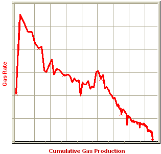
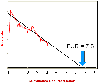
Typically, decline analysis is conducted on a plot of rate versus time or rate versus cumulative production (as shown in figure above). The most commonly used trending equations are those first documented by J.J. Arps (1945). The following figure demonstrates a match trend and extrapolation to the EUR.

Figure 2: Rate versus cumulative gas production

Historical Background

J.J. Arps was an American geologist who published a mathematical relationship for the rate at which oil production from a single well declines over time (1945). His paper made several references to existing methods and theory about decline analysis. References included Arnold and Anderson (1908), W.W. Cutler (1924), H.N. Marsh (1928), and R. E. Allen (1931).

Many contemporary published papers have tried to investigate or modify the Arps decline based on theoretical derivations. However, after 70 years, the original method is still widely in use.

Practical Decline Analysis Key Points

All production can be characterized as having an initial transient flow period followed by a boundary-dominated flow period. During the transient period, the reservoir pressure at the flow boundary remains constant at the initial reservoir pressure and the flow boundary moves outward from the well through the reservoir. This portion of a well’s flow is characterized by very high decline rates. When the flow boundary reaches an actual reservoir boundary, or meets with a flow boundary of another well, the reservoir pressure begins to decline and the well enters the boundary-dominated flow period. It is in this period that traditional decline methods (i.e. Arps) can be used.

The transient flow period can last for time periods from several minutes to several years, depending upon permeability and the areal extent of the reservoir. For most conventional production, the transient flow period ends after a few days. Tighter reservoirs that have permeability in the 0.5 to 1.0 mD range can have transient periods that last several months. Reservoirs that have even lower permeabilities that require extensive fracture networks can have transient periods that could last for several years.

Once a well has achieved boundary-dominated flow, another important consideration is the sandface flowing pressure. For the period of production included in the decline analysis, the sandface flowing pressure must be relatively constant before a reliable set of decline parameters can be extracted. Factors that affect sandface flowing pressure are rate controlled wells, changing wellhead backpressure, changing wellbore configurations, and liquid loading.

Decline Theory

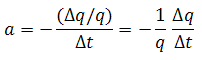
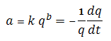
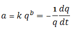
The theory of all decline curve analysis begins with the concept of the nominal (instantaneous) decline rate (a), which is defined as the fractional change in rate per unit time:

Another way of representing the decline rate is based on rate (q) and the decline exponent constant b.

When production is plotted as flow rate vs. time, the nominal decline rate is equal to the slope at a point in time divided by the rate at that point.

Figure 3

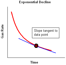
The behaviour of the production data can be characterized based on the way in which the nominal decline rate varies with rate, based on the value of the decline exponent constant b.

• Exponential — b = 0
• Hyperbolic — b is a value other than 0 or 1
• Harmonic — b = 1

Exponential

For the exponential case, b = zero. The decline rate can be shown as:

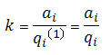
Where k is a constant equal to a / qb at initial conditions:

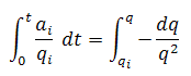
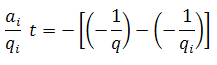
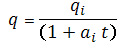
As the decline rate remains constant, the integration of the equation for decline rate results in:

Therefore, a plot of flow rate vs. time, with rate set to a logarithmic axis, will result in a straight line.

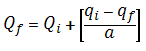
The cumulative production is defined as:

Therefore, a plot of flow rate vs. cumulative production will result in a straight line.

Hyperbolic

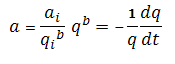
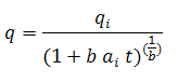
For the hyperbolic case, b is equal to any number between zero and one. The decline rate can be shown as:

Where k is a constant equal to a / qb at initial conditions:

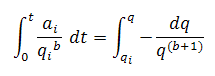
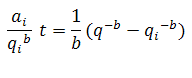
As the decline rate is not constant, the substitution and integration of the equation for decline rate results in:

Substituting

 

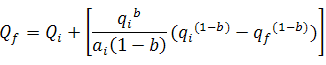
The cumulative production is defined as:

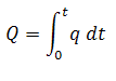
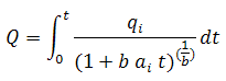
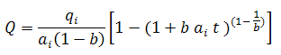
Substituting

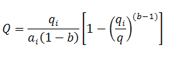
It is noted that neither a plot of flow rate vs. time or flow rate vs. cumulative production will result in a linear relation (regardless of whether rate is set to a Cartesian or logarithmic axis).

Harmonic

The harmonic case is a special case of the above hyperbolic case, where b is equal to one. The decline rate can be shown as:

Where k is a constant equal to a / qb at initial conditions:

As the decline rate is not constant, the substitution and integration of the equation for decline rate results in:

Substituting

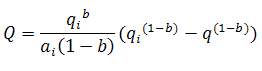
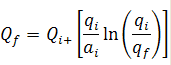
The cumulative production is defined as:

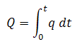
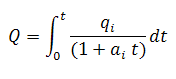
Substituting

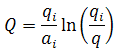
It is noted that a plot of flow rate vs. time will not result in a linear relation (regardless of whether rate is set to a Cartesian or logarithmic axis). A plot of flow rate vs. cumulative production, with rate set to a logarithmic axis, will result in a straight line.

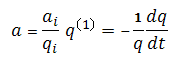
Exponential Decline Rate: Nominal vs. Effective

When production follows an exponential decline, there are two different ways of defining the decline rate: Nominal and Effective.

The first is the nominal decline rate, represented by the symbol "a". The nominal decline rate is defined as:

The nominal decline rate is used to calculate the rate decline at a specific time. For a given time, the equation for rate using nominal decline is:

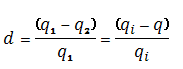
The second is the effective decline rate, represented by the symbol "d". The effective decline rate, for a particular time period (typically one year), is defined as:

The effective decline rate is used to calculate the rate decline for particular time periods. For one time step, the equation for rate using effective decline is:

Note that the time interval is included in the equation for rate using effective decline, but is explicitly stated in the equation for rate using nominal decline.

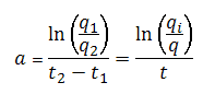
Although the equations for nominal and effective decline rates are different from one another, there is a relationship that will give the same answer for q2 provided the time intervals between q1 and q2 are the same. The relationship between the two is given by:

Note:    The above equation is only valid for the exponential equations.

The difference between the two decline rates is illustrated below. In effect, the nominal decline rate is related to the instantaneous slope of the line, whereas the effective decline rate derives from the chord segment approximating that slope. Also, the rate by which the slope is divided is different - instantaneous rate (q) is used in the case of nominal decline, whereas the preceding rate (q1) is used in the case of effective decline.

Figure 4: Comparison of Nominal Decline and Effective Decline

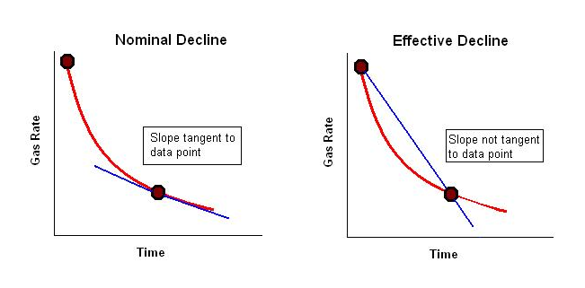
The effective decline rate typically arises when dealing with flow rate data in tabular rather than graphical format. The difference between the nominal and effective decline rates is very small when the nominal decline rate is small, but as the nominal decline rate gets larger the difference between the two increases. It is therefore important to use these values correctly.

Modified Hyperbolic Decline

Extrapolation of hyperbolic declines over long periods of time frequently results in unrealistically high reserves. To avoid this problem, it has been suggested that at some point in time the hyperbolic decline be converted into an exponential decline (Robertson). Thus, assume that for a particular example, the decline rate starts at 30% and decreases through time in a hyperbolic manner. When it reaches a specified value, 10% for example, the hyperbolic decline can be converted to an exponential decline, and the forecast continued using the exponential decline rate of 10%.

Limited Decline Rate

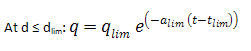
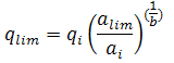
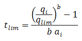
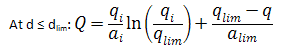
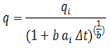
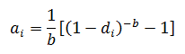
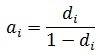
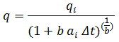
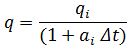
The limited decline rate begins as a hyperbolic decline curve and transitions into an exponential decline curve at a specified limiting effective decline rate, dlim. The limiting effective decline rate is converted to a limiting nominal decline rate, alim, and the following rate – time equations are applied in the analysis:

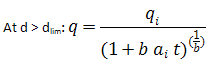
where:

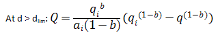
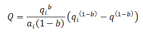
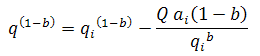
The limited decline rate can also be expressed as rate – cumulative production using the following equations.

For b > 1:

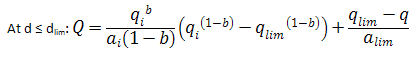
For b = 1:

Values of b > 1

A value of b = 0 corresponds to exponential decline, values of b >0 and < 1 correspond to hyperbolic decline, and a value of b = 1 corresponds to harmonic decline. Values of b >1 are not consistent with decline curve theory, but they are sometimes encountered, and their meaning is explained below.

Decline curve analysis is based on empirical observations of production rate decline, and not on theoretical derivations. Attempts to explain the observed behaviour using the theory of flow in porous media lead to the fact that these empirically observed declines are related to boundary-dominated flow. When a well is placed on production, there will be transient flow initially. Eventually, all of the reservoir boundaries will be felt, and it is only after this time that decline curve analysis becomes applicable. During boundary-dominated flow, the value of "b" lies in the range of 0 to 1, depending on the reservoir boundary conditions and the recovery mechanism.

Occasionally, decline curves with values of b > 1 are encountered. Below are some reasons that have been presented to explain this:

• The interpretation is wrong, and another value of b < 1 will fit the data.
• The data is still in transient flow and has not reached boundary-dominated flow.
• Gentry and McCray (1978), using numerical simulation showed that reservoir layering can cause values of b > 1.
• Bailey (1982) showed that some fractured gas wells exhibit values of b > 1, sometimes as high as 3.5.

Arps Production Decline Equation Summary

Type	Exponential Decline	Hyperbolic Decline	Harmonic Decline
	Decline is constant b=0	Decline is proportional to a fractional power (b) of the production rate 0 < b< 1	Decline is proportional to production rate b = 1
Rate-Time
Rate-Cumulative
EUR

Goodness of Fit

Whenever the decline curve is created to approximate production data, you may want to have a quantitative way to evaluate how good the fit is. There are various metrics that can be used to estimate goodness of fit. In Harmony, R² is reported (this statistic is also known as the coefficient of determination).

R² is calculated using the following equations:

For decline curves created on the q vs t plot:

For decline curves created on the q vs Cum plot:

where:

• i: is the index of summation, and summation is done for all data points after the analysis start date
• q_i,p: is the i-th rate (based on given production data)
• q_i,c: is the i-th rate (based on decline-curve approximation)
• : is the average for all rates q_i,p used in calculations
• : is the average for all used in calculations

Note:   The closer R² is to 1, the better the fit.