Flowing Material Balance (FMB) Analysis Theory

The determination of reserves is a fundamental calculation in reservoir engineering. The material balance method uses actual reservoir performance data and therefore is generally accepted as the most accurate procedure for estimating original hydrocarbons-in-place. In order to generate a traditional material balance plot, the well is shut in at several points during its producing life to obtain the average reservoir pressure. However, this is sometimes impractical, and usually the duration of the shut-in is often not long enough to obtain an accurate measurement. The flowing material balance uses the concept of boundary-dominated flow or pseudo-steady state flow, as well as flowing pressures and rates to calculate original hydrocarbons-in-place.

Pseudo-Steady State

The flow of hydrocarbons through a porous medium can be divided into transient and boundary-dominated flow periods. When a well has reached boundary-dominated flow, its behaviour is governed by the pseudo-steady state equations. When a reservoir is in pseudo-steady state flow and the flow rate is constant, the pressure at all locations in the reservoir declines at the same rate. The diagram below depicts pressures in the reservoir at all locations where the wellbore is located at the left and the exterior boundary of the reservoir at the right. Each of the lines, one, two or three represents the pseudo-steady state pressure in the reservoir when the well is flowing at a constant rate. The pressure decline from time one to time two is the same throughout the reservoir as the curves are parallel.

The traditional material balance method would be to shut in the well several times during the productive life of the reservoir, and let the pressure stabilize to an average pressure p1. Similarly, the pressure profile in the reservoir at later times would result in shut-in average reservoir pressures of p2 and p3. It is evident that the drop in pressure from p1 to p2 to p3 is the same as the drop in pressure at any selected point along curves one, two or three. A convenient point for analysis could be at the wellbore. Remembering that curves one, two, and three represent a flowing well, it is evident that a plot of the flowing wellbore pressure (pwf1, pwf2, pwf3) should be parallel to a plot of the average reservoir pressure (p1, p2, p3).

In a flowing situation, the average reservoir pressure clearly cannot be measured. However, as demonstrated above, in a stabilized flow situation, there is very close connectivity between well flowing pressures (which can be measured) and the average reservoir pressure. The pressure drop measured at the wellbore while the well is flowing at a CONSTANT rate is the same as the pressure drop that would be observed anywhere in the reservoir, including the location which represents average reservoir pressure. This is true ONLY if pseudo-steady state conditions are present, meaning all boundaries have been reached and the rate of withdrawal is constant for the period of time that pwf1 through pwf3 were measured.

Gas

The items below apply to gas entities.

Variable Rate Flowing p/Z**

Most gas wells do not have extended periods of constant rate production. Thus the above concepts can't be directly applied. A typical gas well may have a production profile as shown below.

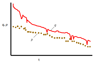
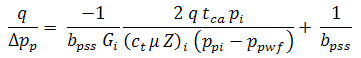
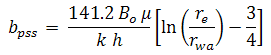
With the above profile, we cannot assume a constant pressure difference between average reservoir conditions and flowing conditions. We know that during boundary-dominated flow:

where:

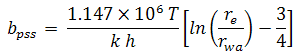
bpss represents the pressure loss due to the steady-state inflow of gas, and is assumed to be constant over time.

For a variable rate system, the equation above clearly shows that the difference between reservoir p/z and flowing p/z is not constant, but rather is a function of flow rate.  Since the flow rate is known, we need only to determine the value of bpss, using some independent method.  Note that the value of bpss did not have to be explicitly determined for the constant rate case because the total value of "q bpss" (the product of flow rate and bpss) was determined graphically.

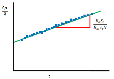
One way to obtain a reliable estimate of bpss is to plot the production and flowing pressure data in the following manner:

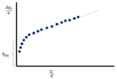
The straight line portion of this graph represents boundary dominated flow, and the y-intercept is bpss. This value of bpss may then be used in the above equation to calculate the average reservoir pressure. Note that the value of bpss is always subject to interpretation as it depends on proper identification of the stabilized (straight line) section of the above graph.

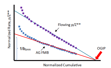
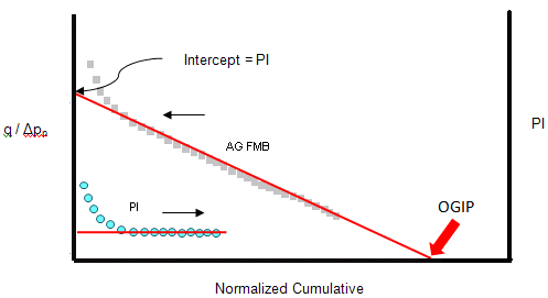
Alternatively, b_pss can be obtained from the Agarwal-Gardner flowing material balance analysis plot. As shown below, 1/b_pss is the y-intercept on that plot. Obtaining the value from the best fit straight line interpretation below, the flowing p/z** values can be calculated.

Agarwal-Gardner Normalized Rate

An alternative to the flowing p/z plot is the Normalized Rate / Normalized Cumulative analysis. The normalized rate approach applies to both oil and gas reservoirs, and works for constant- or variable-rate systems. Its advantage is its flexibility and ease of use. Its primary drawback is that the resulting analysis plot is not as intuitive as that of the flowing p/z.

The procedure is similar to the pseudo-steady state approach, but involves plotting the inverse of the pseudo-steady state equation, so that a declining trend is produced. The normalized rate is plotted against the normalized cumulative. A line is then drawn through the best fit of the points, and the x-intercept is the original gas-in-place. The governing equation for the straight line equation for the Agarwal-Gardner analysis is:

where:

and:

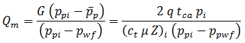
To calculate the average reservoir pressures, use the general material balance equation below, and first assume a value for original gas-in-place. This is an estimate and can be obtained from volumetrics, modeling, or some other analysis.

The step-by-step procedure for generating the Agarwal-Gardner analysis for a gas well with varying flow rate is:

1. Convert initial pressure to pseudo-pressure.

2. Convert all flowing pressures to pseudo-pressures.

3. Assume a value for original gas-in-place.

4. Calculate p/z** from the general material balance equations.

5. Using lookup tables, find the corresponding average reservoir pressure.

6. Convert average reservoir pressure to pseudo-pressure.

7. Using the equations above, plot a graph of normalized rate versus normalized cumulative.

8. Draw a straight line through the best fit of the data points. (The intercept on the x-axis gives original gas-in-place.)

9. Using this new value of original gas-in-place, repeat steps 4-8 until the original gas-in-place converges.

Productivity Index

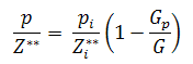
The productivity index of a well is a measure of the production rate achievable under a given drawdown pressure, which is the difference between the average reservoir pressure and the flowing bottomhole pressure. Defined as the flow rate per unit pressure drop, the productivity index gives an indication of the production potential of a well.

From the pss equation above:

therefore:

From a reservoir point of view, well management primarily depends on the well productivity index, which is in turn dependent on rock and fluid properties. One of the principal causes of the reduction in well productivity is formation damage around the wellbore. For flowing material balance analysis, when the "correct" original gas-in-place is found, the productivity index dataset should be relatively flat, indicating that the productivity index is not drastically changing over time.

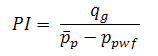
As can be seen above, the productivity index equation is very similar to the traditionally used simplified AOF equation, shown below. The major differences being that:

• The above productivity index is written rigorously using pseudo-pressures and the AOF equation uses the simpler pressure squared method.
• The AOF equation introduces the concept of laminar/turbulent flow using the exponent 'n'.

Assuming n = 1:

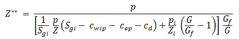
Advanced Gas Material Balance Techniques - p/Z**

The graphical simplicity of the conventional p/Z material balance analysis makes it quite popular. Developed for a "volumetric" gas reservoir, it assumes a constant pore volume of gas and accounts for the energy of gas expansion. However, advanced methods have been developed to account for other sources of energy such as the effects of formation compressibility, residual fluids expansion, and aquifer support. Furthermore, these methods can also account for other sources of gas storage such as connected reservoirs, or adsorption in coal/shale. The flowing material balance analysis accounts for all of these effects if required. The formulation for the calculation of p/Z** is highlighted below:

where:

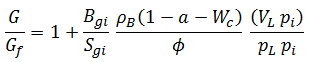
and total compressibility is defined as:

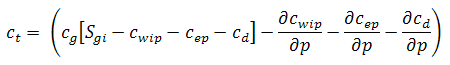
The table below outlines the formulations for the total compressibility equations for all reservoir types.

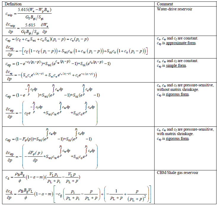
Note:   For more information, see Moghadam et al. (2009).

Oil

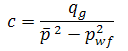
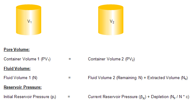
The basis for the flowing material balance of oil comes from both the definition of compressibility and the steady state inflow equation. Compressibility is defined as:

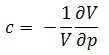
This equation shows that compressibility is defined as the relative change in fluid volume per unit change in pressure.

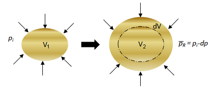
The above schematic demonstrates that as pressure is reduced, the fluid will expand to occupy a larger volume such that V2 > V1. However, most reservoirs can reasonably be expected to have a constant pore volume such that PV1 = PV2. Consequently, as we produce fluid from a reservoir, the remaining fluid in the reservoir expands to fill the pore volume and so the reservoir pressure is reduced.

Production from an undersaturated* oil reservoir can be visualized as follows:

* There is no free gas since the reservoir pressure is greater than the bubble point pressure of the oil.

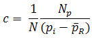
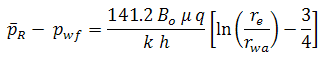
Thus the change in pressure is the difference between the initial reservoir pressure and the average reservoir pressure, and the change in volume is the produced volume up to that point in time. Knowing that the initial volume is the total oil-in-place, these terms are applied to the compressibility equation.

Combining the above relationship with the pseudo-steady equation, rearranging and substituting for material balance time gives the following:

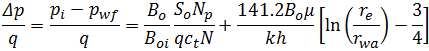
The above equation clearly illustrates the relationship between initial pressure, flowing pressure, and rate.

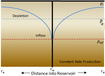
From the figure above, it is apparent that the pseudo-steady state equation is the sum of two distinct pressure loss components:

Pressure loss due to depletion:

Pressure loss due to inflow:

The advantage of the pseudo-steady state formulation is that the average reservoir pressure is eliminated during the addition of pressure loss due to depletion and pressure loss due to inflow, and thus is not explicit in the equation. This is an obvious advantage, because the average reservoir pressure is an unknown. Since both terms (pressure loss due to depletion and pressure loss due to inflow) are functions of rate, we can simplify the  pseudo-steady state equation as follows:

where:

A graph of normalized pressure vs. time produces a straight line, the slope of which provides the original oil-in-place. This is the most basic form of flowing material balance, and is directly applicable to undersaturated oil reservoirs. In well testing, this procedure is commonly referred to as a Reservoir Limits Test.

However, to make it more intuitive and similar to a gas material balance plot, the pseudo-steady state equation above is rearranged to the following:

Plotting normalized rate vs. normalized cumulative (similar to the Agarwal-Gardner plot), the following plot is derived, where the x-intercept is equal to the original oil in place.

The above equation and associated figure describe the flowing oil material balance analysis for a volumetric circular reservoir.

Accounting for Variation in Oil Properties

The derivation for oil Flowing Material Balance (FMB) given above is valid under the assumption that the variation of oil and rock properties (c_t, B_o, μ_o, and k) with pressure is negligible. That assumption is valid for some cases, but sometimes (for example, for oil with high gas content, or for cases with pressure-dependent rock properties), it is important to accurately account for variations in oil and rock properties.

This is done similarly to Agarwal-Gardner FMB analysis for gas.

Oil pseudo-pressure is defined as:

Total pseudo-pressure drop can then be written in terms of oil pseudo-pressure and can be presented as:

Under conditions of pseudo-steady state, the pressure drop due to Darcy flow and flow rate are related by:

Where Constant is defined by reservoir and completion geometry, but does not change with pressure. Using rules of integration, this can be re-arranged as:

Therefore, pressure drop due to Darcy flow in terms of oil pseudo-pressure can be expressed as:

Where b'_pss does not vary with pressure.

Using this formulation for pressure drop due to Darcy flow, total pressure drop can be presented as:

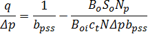
Dividing both sides by Δp_po b'_pss and re-arranging we get:

(Note that we added N to both the numerator and denominator of the last term.)

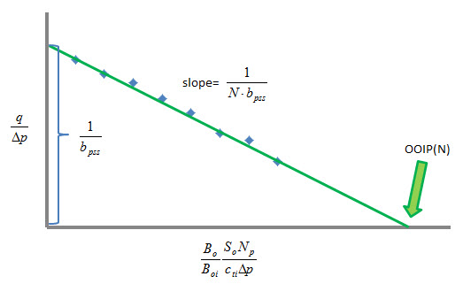
This equation is used to create a plot for oil FMB analysis that accounts for variation of oil and formation properties.

The y-values for each data point can be readily calculated based on production data:

To calculate x-values, use an iterative procedure:

1. Estimate a value for oil in place, N_guess.

2. Calculate the average reservoir pressure based on N_guess, known production data, and using rigorous material-balance calculations.

3. Calculate x-values:

4. Generate an FMB plot (y-values vs. x-values).

5. Draw a straight line through the data points corresponding to boundary-dominated flow (the late portion of the data).

6. The y-intercept of the line equals 1/b'_pss, and the slope of the line equals 1/(Nb'_pss); therefore N can be calculated.

7. Compare the calculated N with N_guess. If they are not equal, set the next N_guess to the value calculated in step 6, and return to step 1.

8. Iterate until N = N_guess.

This approach is described by Stalgorova and Mattar (2016).