Single vs. Multiple Well Analysis
All of the methods used in RTA apply to single well analysis only. When considering the production of multiple wells in a field and/or reservoir, the available methods are as follows:
- Empirical - Group production decline plots
- Material Balance Analysis – Shut-in data only
- Reservoir Simulation
- Semi-analytic production data analysis methods (Blasingame et al.)
The first step in analyzing multiple wells is to identify the objective of the analysis. The following is a list of situations where multiple well analyses is required:
Situations where high efficiency is required:
- Scoping studies / A & D
- Reserves auditing
Single well methods don’t apply:
- Interference effects evident in production / pressure data - Wells producing and shutting in at different times
- Predictive tool for entire reservoir is required
- Complex reservoir behaviour in the presence of multiple wells (multiphase flow, reservoir heterogeneities)
The vast majority of production data can be analyzed effectively without using multi-well methods. The following is a list of situations where single well analysis would suffice:
- Single well reservoirs
- Low permeability reservoirs (pressure transients from different wells in reservoir do not interfere over the production life of the well)
- Cases where "outer boundary conditions" do not change too much over the production life of the well (wide range of reservoir types)
Identifying Interference


Blasingame et al. Interference Analysis
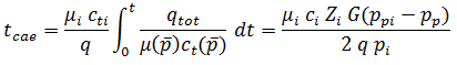
Blasingame et al. Interference Analysis extends the concept of single well decline analysis using typecurves to a multi-well pool. The process involves analysis of the single well normalized rate response (q/Dp), but plotted against a material balance time that includes the effect of the offset wells in the reservoir.

Blasingame Typecurve Matching: Multiple Well Pools
For Blasingame typecurve analysis in multi-well pools, the material balance time function is adjusted to account for total pool production as follows:

Oil Wells

Gas Wells
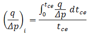
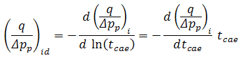
The three rate functions are as follows (defined exactly the same as for single well analysis, except that material balance time is replaced by total material balance time):
Normalized Rate
Oil Wells

Gas Wells

Rate Integral
The rate integral is defined at any point in the producing life of a well, as the average rate at which the well has produced until that moment in time. The normalized rate integral is defined as follows:
Oil Wells
Gas Wells

Rate Integral Derivative
The rate integral derivative is defined as the semi-logarithmic derivative of the rate integral function, with respect to material balance time. It is defined as follows:
Oil Wells

Gas Wells
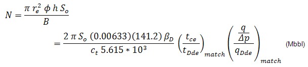
Calculation of Parameters
The calculation of parameters for the multi-well pool case is very similar to that of the single well typecurve analysis. However, total material balance time (and total material balance pseudo-time) is used in place of material balance time. In addition, a new variable βD is introduced. The dimensionless group reD / βD replaces reD as the typecurve matching parameter for the multi-well case. βD is defined as the ratio of total pool production to individual well production. Strictly speaking, this will vary with time; however it can be approximated as:
![]()
The following reservoir parameters are calculated in the same manner as in the single well typecurve analysis:
- Permeability (k)
- Skin (s)
- Fracture half-length (xf)
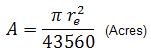
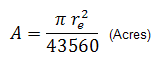
- Area (A)
- Original gas-in-place (OGIP) / Original oil-in-place (OOIP)
The parameters OGIP / OOIP and area, however, apply to the entire pool rather than just the individual well.
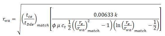
Typecurve Matching Equations: Multi-Well Radial
Oil Wells
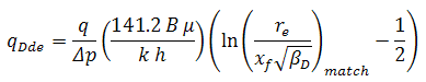
We define dimensionless decline rate accounting for total pool production (qDde) as follows:

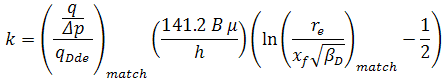
Permeability (k) is obtained from rearranging the definition of qDde:

Now, dimensionless decline time accounting for total pool production (tDde) is defined as follows:

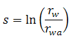
Solve for apparent wellbore radius (rwa) and skin as follows:

Solve for reservoir effective radius (re) from the product of qDde and tDde:


Gas Wells
Permeability (k) is obtained from rearranging the definition of qDde:


Solve for apparent wellbore radius (rwa) from the definition of tDde:


Solve for reservoir effective radius (re) from the product of qDde and tDde:


 (Bscf)
Typecurve Matching Equations: Multi-Well Fractured
Oil Wells
Permeability (k) is obtained from rearranging the definition of qDde:
Solve for fracture half-length (xf) from the definition of tDde:
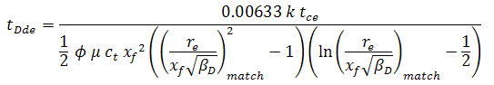

Solve for wellbore effective radius (re) from the product of qDde and tDde:


Gas Wells
Permeability (k) is obtained from rearranging the definition of qDde:


Solve for fracture half-length (xf) from the definition of tDde:
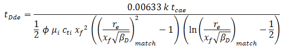

Solve for wellbore effective radius (re) from the product of qDde and tDde:

 (Bscf)
Multi-Well Pools
It is common practice to apply decline curve analysis to aggregated production from a lease or pool. The extension of decline analysis from a single well to aggregated production from a number of wells is sometimes difficult to justify theoretically. For example, the sum of the flow rates from two wells with exponential decline is not exponential in general, unless both wells have the same decline. However, this concern is lessened, when there are sufficient wells to result in a statistical distribution. Purvis has written two papers in which the decline performance of a pool is studied in a statistical manner.
Most of the difficulty in extending the single well analysis to an aggregate of wells is often due to the inevitable variation in the number of producing wells over time. If the wells have reasonably similar declines, it is suggested that the decline analysis be performed on an "average well per operating day", and that the pool forecast be obtained from the performance of the average well combined with a forecast of the number of producing wells, and adjusted by a factor to account for downtime.
The economic abandonment rate for an aggregate of wells can be misleading. Consider, for example, the case of three producing wells, two of which are at a rate below the economic limit and one is producing at a high rate. It is very possible that the total rate of the three wells would be higher than three times the economic limit of any one well. Analysis of the aggregate production would result in continuation of the operation of all three wells (because their total flow rate is larger than the aggregate economic abandonment rate). Yet analysis of the individual well rates would clearly show that two of the wells should be abandoned.
Another consideration in multi-well pools is to initialize the production rate of each well to a common start time. This makes it easier to arrive at the "average well" performance.
