A probabilistic analysis works by repeatedly running a hybrid model to generate a range of forecasts. For each run, the values for the majority of the parameters are taken from the base hybrid model, and values for parameters that are uncertain, are drawn from given distributions. As a result, you get a range of forecasts and a distribution for values of expected ultimate recovery (EUR).
Note: This analysis works with your IHS Reservoir™ license.
A probabilistic analysis can be run on any hybrid analysis with valid parameters and a forecast.
If values for some of a hybrid model's parameters are uncertain, but you have some idea about their range and distribution, you can use a probabilistic analysis to account for this uncertainty.

A probabilistic analysis has three tabs: Setup, Dependencies, and Results.
This tab contains parameters for the probabilistic analysis, and cards where you can define the distributions for parameters.
To indicate that a parameter's value is uncertain, click the Add Parameters icon (![]() ), and select the parameter from the drop-down list. A distribution card is added to this tab where you can define the distribution to be used for this parameter.
), and select the parameter from the drop-down list. A distribution card is added to this tab where you can define the distribution to be used for this parameter.
Probabilistic simulation may take a long time, especially if the number of runs is high.
You can set your number of hybrid-model runs in the simulation as follows:
After you add and set up distribution cards for all your uncertain parameters, click the Run Simulation button to start your simulation.

After you add distribution cards for your uncertain parameters, you can select one of these distribution types: normal, log-normal, triangular, or uniform. For more information, see the descriptions below and probabilistic theory.
With some parameters, you can select automatic parameter estimation (APE) from the Distribution drop-down list. For more information, see APE.
By selecting Normal, you can apply a normal distribution to a particular parameter by entering a mean and variance, or a Min (P90) and Max (P10).

Additionally, you can enter a Sample Min and Sample Max for a normal distribution. In this case, the distribution is truncated, and the probability function is adjusted such that the total probability still sums up to 100%. For more information, see truncated distributions.
By selecting Log-Normal, you can apply a log-normal distribution to a particular parameter by entering a mean and variance, or a Min (P90) and Max (P10).

Additionally, you can enter a Sample Min and Sample Max for a log-normal distribution. In this case, the distribution is truncated, and the probability function is adjusted such that the total probability still sums up to 100%. For more information, see truncated distributions.
By selecting Triangular, you can apply a triangular distribution to a particular parameter by entering a minimum, mode, and maximum. The minimum and maximum values define the extent to which the probability density is equal to zero. The mode defines the peak.

By selecting Uniform, you can apply a uniform distribution to a particular parameter by entering a minimum and maximum.

In a typical scenario, you would run probabilistic analysis for a hybrid model that matches historical data. However, after you change the values for uncertain parameters based on a given distribution, the history match is likely to get spoiled. You may want to adjust some other parameters to restore the match. To do this, set the distribution for those additional parameters to APE.
APE iteratively varies the value of a parameter and attempts to minimize the total error between the measured data and the simulated values. When the model uses a rate to calculate pressure, it minimizes the difference between the simulated and measured pressures. When the model uses pressure to calculate rates, it minimizes the difference between the measured and simulated primary fluid rate. Only the primary fluid rate match is minimized.
For each probabilistic run, the best match that APE could find is used to generate a forecast. There is no filtering of these results based on the quality of the match found by APE.
Example:
Assume you have a base hybrid model that matches historical data, and this model has xf = 120 ft. In reality, you are not certain if the value of xf is indeed 120 ft, but based on the available information, you can confidently assume that xf is varying between 80 ft and 160 ft, and can set the distribution for xf to Normal.
For each run within the probabilistic analysis, Harmony picks a value for xf based on the given distribution. Simply changing the value for xf results in runs that do not match the historical data.
To mitigate this problem, set the distribution for kSRV and/or kmatrix to APE. In this case, for each run within the probabilistic analysis, Harmony picks xf based on the given distribution, and then runs APE on kSRV and/or kmatrix (keeping xf at the value drawn from the given distribution).
Using APE for some of the model's parameters ensures that all probabilistic runs match historical data as closely as possible. However, it is important to keep in mind that when using APE, each probabilistic run requires many runs of the hybrid model; therefore, the overall simulation time increases significantly.
When running APE on a certain parameter, you can set user-defined limits for it by clicking the View Defaults and Limits button ( ) to the right of the parameter in the base model.
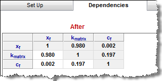
After values are sampled during simulation, they are displayed in this tab where relationships between any of the uncertain parameters can be entered. For example, if you know that the porosity and permeability in the reservoir are proportional, a correlation coefficient can be entered to represent this relationship. These values must be between -1 and 1, and must be entered in the field that intersects the two desired variables.

The lower plot displays a cross-plot for the variables you select in the above table.

If you set up more than two parameters in the Setup tab, correlation coefficients between each pair of parameters are not independent. After you enter the correlation coefficients, a Correct the matrix button appears. Click this button to adjust the coefficients you enter, such that the coefficients for each pair become consistent.

In this tab, a dashboard view is displayed.

After your simulation runs are complete, you can export your data to Excel by clicking the Export Data icon ( ).
).
To take the varied parameters from the first probabilistic run and populate them in the base model in the Hybrid Model pane, click the ![]() icon.
icon.
Tip: If you see a warning that the "Source model changed", you may need to re-run the simulation on the Setup tab, or the base hybrid model to clear the warning. The base model can get out-of-date when auto-calculate is deselected (see AutoCalc) and you make changes to parameters (that is, the results become out-of-date).
Filter — you can filter the cases / runs used in determining the P90, P50, and P10 based on a cut-off for the average error (Eavg) of each run. Therefore, in every model's run, an average error is determined: it is the average of the error between each measured data point and the synthetic one calculated by the model at that point. The average error is intended to give a sense of the quality of a match. This is true of any hybrid or analytical model, as well as the runs calculated for the probabilistic cases. When you are viewing the variation of forecast outcomes based on a range of model parameters, it is useful to be able to exclude any randomly selected parameter sets in the defined range that produce a “bad” match. Above the Rate vs Time plot, there is a drop-down list. By selecting Add Filter, you can type in a value for the error cut-off (between 0 and 1). Or you can select the default value of None (1.5 times the average of all the Eavg values from the probabilistic runs). When you type a value (instead of selecting the default None setting), all the table results and forecast ranges displayed only include runs that have an Eavg below this value.
Tip: Any Eavg cut-offs you enter are saved within your current session, but are not saved to the database.
By default, these views are displayed from the upper left to lower right:


After the probabilistic simulation is complete, Harmony creates P10, P50, and P90 forecasts based on all the successful runs within the probabilistic simulation. Remaining recoverable (RR) volumes and EUR volumes are calculated for these forecasts. For more information on calculations, see percentile calculations.
In some regards, P10, P50, and P90 forecasts (also called percentile forecasts) can be treated as separate analyses in Harmony. For example, you can:


IHS Harmony Enterprise™ 2017.3 | Last revised: October 18, 2017
Copyright © 2017 IHS Markit Ltd. All rights reserved.