Decline analysis

The decline analysis uses the conventional Arps’ decline method and generates forecasts of future production rates, and the estimated ultimate recovery (EUR) of reserves. For additional information on theory and concepts, see decline analysis theory. When you add a decline analysis (see analyzing an entity), Harmony Enterprise automatically selects the best subset of your data (90% of your data points) for an initial best fit.

Note:

This analysis works with your Harmony Forecast™ license.

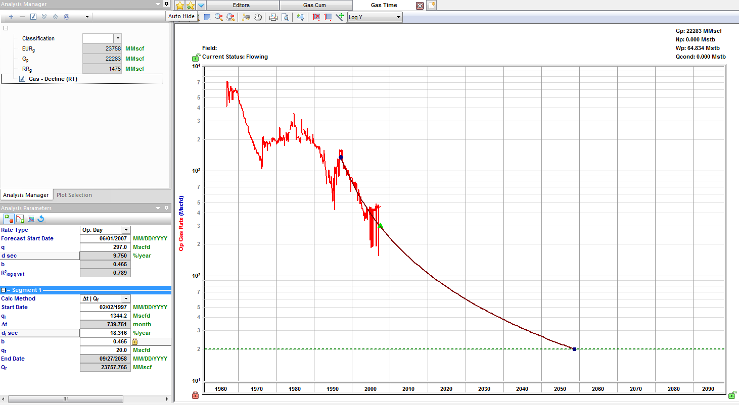
Analysis Parameters pane

After you add your decline analysis, the selected analysis (highlighted in purple) has its detailed parameters displayed in the Analysis Parameters pane located below the Analysis Manager pane (the default setting).

Harmony Enterprise automatically fits (best fits) your decline curve based on:

• recent trends.
• rate data. It is able to handle shut-ins, and exclude these data points from the best fit.
• If you have anomalies in your data, a local outlier factor algorithm is used to determine which data points are considered outliers to be excluded from the initial best fit.

In order for the auto-fit algorithm to work, at least six months of data is required. If there is not enough data, all of the data points are selected, and a decline curve is generated based on the data that is available. Harmony Enterprise automatically selects the best subset of your data for an initial best fit.

In this pane, you can specify / view the following settings and parameters:
(The parameters that are displayed depend on if the analysis was created on a rate-time (RT) or rate-cumulative (RC) production plot.)

• Rate Type — select calendar rate (Cal. Day) or operator rate (Op. Day) from the drop-down list. For more information, see rate type.
• Forecast Start Date — the decline curve in Harmony Enterprise includes a "best fit" of historical data followed by a forecast section. The Forecast Start Date (FSD), highlighted by a small green triangle, defines the beginning of the forecast. For more information, see forecast start date.
• q — the production rate at the FSD.
• d _sec — the effective decline rate at the FSD. It can be toggled to d_tan, or a nominal decline rate.
• b — the decline exponent at the FSD.
• R² — an indication of the precision of the history match. It is reported as R²_{log q vs t} on a rate-time (RT) plot, and R²_{q vs Q}on a rate-cumulative (RC) production plot.

Rate type

The rate type can be either calendar rate or operated rate, which you can select from the drop-down list at the top of Analysis Parameters pane. However, you first need to select the rate type you want from the Plot Selection tab, which is located next to the Analysis Manager tab (by default).

Note that if you select both the calendar rate (for example, Cal Gas Rate) and operated rate (for example, Op Gas Rate), they appear as separate axes on your plot. After you select the rate type to place your decline analysis on, the decline curve is placed on that rate history. The decline parameters do not change, but the precision of your match, indicated by R², does consequently change. Also, the point selection tool for best-fitting () is only active on the selected axis.

Forecast start date

The forecast start date (FSD) defaults to the last data point in the production history (or the active reference date, if it is set to an earlier time). However, you can change this date, which updates the corresponding rate (q), effective decline rate (d_sec), and the decline exponent (b) reported below that date.

Multiple segments

You can add multiple segments (see analysis parameters toolbar) to your decline analysis, and under each segment, you can change parameters and the calculation method for that segment.

Under each segment's tab, you can specify / view the following parameters:

• Calc Method — select the decline parameters you want to enter as inputs, and the parameters to be calculated by Harmony Enterprise. For more information, see decline calculation methods.
• Start Date — sets the onset of the decline in a segment. For the first segment, it is defined by the time of the historical (best fit) portion when the decline curve begins.
  
  
  • In each best fit of production data, the Start Date defaults to the first selected point, and is highlighted by a small blue square. By default, Harmony Enterprise selects the last 50% of the data for curve-fitting, but you can change this percentage by clicking the Point Selection Tool icon ().
• q_i — the initial production rate and is reported / specified at the Start Date.
• d_{i sec} — the initial effective decline rate and is reported / specified at the Start Date. You can toggle this parameter to show either d _{i tan} or a_i (nominal decline rate).
• Δt — the duration of the decline segment.
• q_f — the final forecast rate (abandonment rate), and is initialized from the settings defined in the Options dialog box (see decline options). However, you can manually modify this rate by entering a new value. When a decline is added to a group, the abandonment rate uses the value in the Options dialog box multiplied by the number of producing wells.
• b — the decline component. The initially reported b value results from the best fit of the selected historical data to a hyperbolic decline, unless a fixed b value is defined in the Options dialog box.
  
  
  • The b value can be automatically updated each time you change the historical portion of the fit, if you have the yellow lock icon () open. If this icon is in a locked position (), your b value is locked and changing the selected history does not impact the reported b value.

Analysis Parameters toolbar

The Analysis Parameters toolbar has the following key icons:

• Show / Hide Results Line — shows (default setting) or hides the dashed line on the plot that represents the abandonment rate for the decline analysis and the d_lim transition.
• / Add / Remove Segment — adds a new segment to the end of the existing decline forecast, or removes the last segment. When you add a new segment, this is how Harmony Enterprise initializes that segment:
  
  
  • Nominal decline rate (a) — the beginning of the new segment and the end of preceding segment are equal.
  • q_i of the new segment is set to q_f of the preceding segment.
  • The b value of the new segment is the same as that of the preceding segment, and a duration of 60 months is initially applied.

• Fit Decline to Forecast and Selected Production Points· — clears your historical data selections (the decline "best fit") and uses the data points for the forecast you select. Any additional points you manually select are included in the "best fit" as well. If you select None from the drop-down list, your forecast data is not included in best fits.
• Tip: This option works on these forecast types: stretched, Duong, WOR total fluid, custom, ratio, typecurve, analytical, hybrid, and the unconventional reservoir model. When best-fitting data, you can control when the b value (slope) should be minimized. For more information, see b value minimization in the Options dialog box.
• Reinitialize Segment — for reinitialization of a segment, you can select one of the following options from the drop-down menu:
  
  
  • Reinitialize Segment — the nominal decline rate (a) at the beginning of a new segment and end of its preceding segment are set to be equal to ensure there is a smooth transition between the two segments. Also, q_i of the new segment, and q_f of the preceding segment, are set to be equal. If you have more than two segments, this reinitialization rule applies to all of the segments.
  • Reinitialize Segment q_i — only the q_i of new segments, and the q_f of their preceding segments, are set to be equal to attach the segments together.
• Reset decline to initial state — resets the plot to the default best fit (initial auto fit). Note that if you changed the dlim Exp field in the Options dialog box, clicking this icon resets the plot to the current value in this field.

Decline calculation methods

After you have created your decline analysis, you can modify the parameters by entering new values. As the parameters are changed, calculated values and the forecast line on the plot are updated. To change which parameters are specified, you can change your calc method.

The table below lists which values are specified (denoted by S), and which are calculated (denoted by C), in different calc methods. For special parameters or calc methods, some parameters are marked as not applicable (n/a).

Calc Method	qi	Δt	di	b	qf	Qf	dlim
Δt | Qf	S	C	S	S	S	C	n/a
Δt | di	S	C	C	S	S	S	n/a
Δt | qf	S	C	S	S	C	S	n/a
qf | Qf	S	S	S	S	C	C	n/a
di | Qf	S	S	C	S	S	C	n/a
di | qf	S	S	C	S	C	S	n/a
di | b	S	S	C	C	S	S	n/a
Fixed Rate	S	S	n/a	n/a	n/a	C	n/a
dlim - Δt | Qf	S	C	S	S	S	C	S
dlim - qf | Qf	S	S	S	S	C	C	S
dlim - Δt | qf	S	C	S	S	C	S	S
Inclining Rate	S	C	S	n/a	S	C	n/a

• Fixed rate — this calculation method can be used to create a constant rate forecast. When you switch to this calc method, the previous q_i and Δt are maintained. These are the only parameters that can be changed for this forecast type.
• d_lim — when a decline forecast has a b value greater than 0, the decline rate (or slope at a given point on the curve) decreases through time. The decline rate can become very small, resulting in a very long forecast and sometimes an unreasonable EUR. The d_lim calc method provides a way to limit this by setting a minimum decline rate (d_lim). After this minimum decline rate is reached, the forecast proceeds with a b of 0 (a constant decline rate, or exponential decline), and a vertical dashed-green line displays the transition between the two decline regimes.
  
  
  • The limiting effective decline rate can be toggled between exponential (d_{lim exp}) and hyperbolic (d_{lim hyp}). This defines whether the nominal decline rate (at the time of transition from the hyperbolic decline to the exponential decline) should be calculated using the b value of the hyperbolic, or exponential decline regimes.
• Inclining rate — this method can be used to create a segment with an increasing rate. The b value is forced to remain at 0. The q_i, d, and q_f are specified. By default, when you switch to this calc method, the q_i is maintained, and the d_i is converted to a negative value (an inclining rate rather than a declining rate). A q_f is initially calculated to set the Δt to 60 months.

Line manipulation

Line manipulations are initiated by clicking (sometimes while pressing the Ctrl or Shift keys) the line itself, or one of the manipulation points for a given segment (start date, forecast start date, or end date). You can cancel your line manipulation by pressing the Esc key. Specific line manipulations are described below.

Tip:

Any time you see "click", this means to left-click your mouse. Right-click actions are specifically mentioned.

• Forecast Start Date, FSD (indicated by a green triangle on the decline line)
  
  
  • Click, grab-and-drag — maintains the shape of the decline line and the b and d values. Enables vertical shifting of the decline line, which results in changes to q and q_i.
    - The segments after the segment containing the FSD are also affected because they are shifting in time / cumulative production.
  • Shift key — pressing the Shift key while dragging enables you to position the FSD along the decline curve, while maintaining the shape of the decline. This changes your Q_f (only on a rate-time Decline worksheet).
    - Positioning of the FSD beyond the historical production is restricted on a rate-cumulative (RC) production decline.
  • Ctrl key — pressing the Ctrl key while dragging enables horizontal shifting (translation) of the decline with time. This impacts the FSD in time on a rate-time (RT) plot, but the decline parameters remain unchanged.
    - If the FSD is located on the second segment, pressing the Ctrl key results in behavior similar to "click, grab-and-drag" on the second segment.
• Start Date (indicated by a blue circle)
  
  
  • Click, grab-and-drag — moves the decline line vertically to change the q_i of the segment. However, it does not change the start date or FSD. The shape of the decline (b and d) line is preserved.
    - Both q_i and q for the segment being manipulated get modified, and all segments following this segment are shifted in time / cumulative production, accordingly.
  • Shift key — pressing the Shift key while dragging extends your forecast back into the historical production. The start date, q_i, and d_i change, but the b value is not impacted.
    - This Shift-key functionality does not apply to a secondary segment.
  • Ctrl key — pressing the Ctrl key while dragging translates the curve along the x-axis. The start date, FSD, and forecast end date advance in time for the first segment.
    - This Ctrl-key functionality does not apply to a secondary segment.
• End Date (indicated by a blue square)
  
  
  • Click, grab-and-drag — enables you to move the end date in time, anchoring to the start date and maintaining the q_f. The b value is maintained, but d_i is updated. If the FSD is contained within the segment, then q and d update as well.
  • Shift key — pressing the Shift key while dragging extends your forecast forward in time, and decreases your final rate (q_f). Your final Q_f increases, but none of the decline parameters change.
  • Ctrl key — visually similar to the grab-and-drag functionality for the end date, but the b value can change with the Ctrl-key functionality.
• Any point on the forecast decline curve (activated when the decline segment turns orange)
  
  
  • Click, grab-and-drag — If the segment contains the FSD, that segment is anchored to the FSD and rotates around while the b value and q_f are maintained.
    - On a segment that does not contain FSD, the decline is anchored to the start date of the segment.
    - If you accidentally place the FSD at the end date of a segment, the decline is anchored to the end date of the segment.
  • Ctrl key — the curvature of the line (the b value) changes.

Decline-line customization

You can customize the width and color of your decline line / curve by right-clicking it.

After you customize your decline line / curve, the modifications are saved and applied to every worksheet that displays this decline.

Harmony Enterprise™ 2018.3 | Last revised: October 22, 2018

Copyright © 2018 IHS Markit Ltd. All rights reserved.