Analytical models are used to validate interpretations and provide production forecasting. For more information, see analytical models theory. Analytical models assume single-phase flow in the reservoir and are available for gas, oil, and water production with the following options:
- Vertical
- Vertical with Fracture
- Horizontal
- Hz Multifrac: Enhanced Frac Region
- Hz Multifrac: General Multifrac
| Note: | This analysis works with your Harmony Reservoir™ license. |
Before you start, make sure that all required information is added to the Harmony Enterprise project. Well production data (rates and sandface pressures) should be populated in the Production editor, and reservoir and fluid properties should be specified in the Properties editor.
We recommend that you perform an analysis prior to using the analytical model because this gives you an idea about which values to use. For example, for conventional wells, a flowing material balance (FMB) gives an estimate for original fluid in-place, and the use of a typecurve analysis provides insight about permeability, skin, reservoir shape / size, and fracture properties. For unconventional wells, an unconventional reservoir analysis can be used to estimate permeability, fracture length, apparent conductivity, and the size of the stimulated reservoir volume.
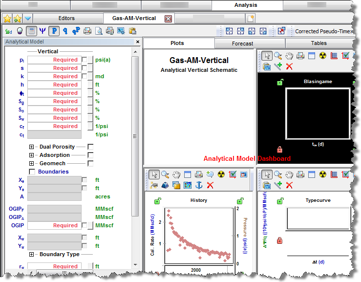
Analytical Model pane
In the Analytical Model pane, enter the required parameters, and select your calculation method from the primary toolbar (CalcP, CalcR, or CalcBoth).
Primary toolbar
There are four toolbars: primary, secondary, Plots sub-tab, and Forecast sub-tab.
The primary toolbar has the following important icons:
-
 Defaults — copies parameters from the Properties editor or other IHS Reservoir worksheets.
 - Or, if you want to copy only one parameter from the analysis, click the View Defaults and Limits button to the right of the field in the Analytical Model pane.
- Note: Parameters copied from the reservoir or another analysis are displayed in a gray font. This indicates that they match the default. You can type new values for any parameter, or change values for some parameters by moving elements of the schematic. Parameters, which do not match the default, are shown in a black font.
-
 Automatic Parameter Estimation (APE) — while APE is running, selected parameters are automatically varied to minimize the error between the simulated pressure / rate and the actual pressure / rate depending on the calculation method (see CalcP, CalcR, and CalcBoth below). The updated simulated pressure / rate is shown on the plots while the calculation is running. For more information, see using APE.
 - Important: The purpose of history matching is to get the calculated pressures / rates to reproduce actual pressures / rates as closely as possible by changing the model's parameters. You can vary model parameters manually, or use APE.
 AutoCalc — recalculates automatically each time you change model parameters.
-
 Synthesize — if you do not click the AutoCalc icon, you must click this icon every time you want to recalculate the model.
  CalcP — calculates the sandface flowing pressure based on measured rate. The pressure is calculated and minimized.
  CalcR — calculates the rate based on given sandface flowing pressures. The rate is calculated and minimized.
  CalcBoth — calculates CalcP and CalcR. Both pressure and rate are calculated and minimized.
  Derivative Options — opens the Options dialog box where you can select Standard (points), Bourdet (cycles), or Difference.
-
 Copy to / Paste from the Clipboard — copies and pastes data from the clipboard.
For a description of common icons, see toolbars.
Secondary toolbar
By default, the secondary toolbar is located to the far right of the primary toolbar. (You can move the icons in the secondary toolbar by clicking the dotted line to the left of the icons.)
By default, the Analytical Model Dashboard displays model schematics and three plots with measured and calculated data. You can change this display (that is, switch plots and their positioning) by clicking one of the Add an Available View icons (upper left, upper right, lower left, lower right) and selecting the plot you want.
![]()
 Add Floating View — opens the plot you select from the drop-down list in its own window.
- Corrected Pseudo-Time — toggles corrected pseudo-time on or off.
Sub-tabs
There are three sub-tabs: Plots, Forecast, and Tables.
Plots
This sub-tab displays your analytical model dashboard, which you can customize using the secondary toolbar. For information on a plot's context menu, see plot options.
Toolbar
This toolbar is located on the Plots sub-tab and has the following important icons:
-
 Reset Plot Attributes — resets your plot attributes to default settings.
 -
 Enable / Disable Square LogLog Plot — changes the range of the x- and y-axes, so that the resolution of a log cycle is consistent between the axes (for example, a log cycle equals 200 pixels on both axes).
 -
 Weigh Data Points — used to emphasize matching to specific data points when using APE (for example, the last part of the production). The cursor changes to a spray gun when clicked. Weighted data points are displayed in a brighter color and are given a 100% weighting; unweighted points are given a 10% weighting. (The weighting is displayed when you hover over the data point.)
 -
 Copy — copies plot data.
 -
 Select Anchor Point — attempts to initialize the anchor to the first measured pressure. If this fails, click the location you want within the plot to set the anchor location. An annotation is shown at the anchor location while this functionality is enabled. Dragging the annotation arrow to a different point updates the calculations. For more information, see anchoring.
 - Tip: The Anchor option is currently only available for analytical models in Calculate Pressure (CalcP) mode.
-
 Hide the Toolbar — hides the toolbar. If you want the toolbar displayed, right-click the plot and select Show Toolbar.
For information on common plot icons, see plot toolbars.
Forecast
This sub-tab has a toolbar, and displays your forecast: options, constraints, and results.
After the model has been populated (either by entering values, or by clicking the Defaults icon) and calibrated to the production and pressure data through history matching (click the Automatic Parameter Estimation icon), production forecasts can be created and compared under a variety of different constraints.
Toolbar
This toolbar is located on the Forecast sub-tab and has the same common icons described in plot toolbars.
Forecast options
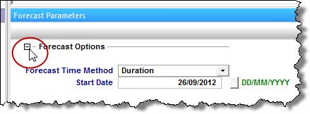
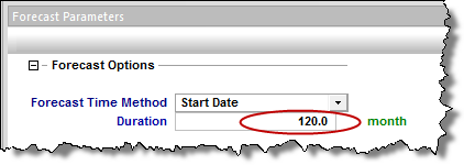
The Forecast Options section is where forecast periods are defined according to either durations (for example, months), or dates.
- Setting the forecast time method to Duration begins a forecast at a specified start date. Forecast periods are then defined in the forecast table according to a length of time (the default is months). For each forecast period, different operating conditions can be specified.
- Setting the forecast time method to Start Date creates a forecast of a specified length of time (the default is months). Forecast periods are then defined in the forecast table according to calendar dates.

If you select Duration from the Forecast Time Method drop-down menu, the Start Date is automatically populated. (You can change this date later, if needed.)

If you select Start Date from the Forecast Time Method drop-down menu, enter a value for Duration (that is, the total length of the forecast).

Forecast Flowing Pressure — when controlling the pressure for forecasting, select whether sandface or wellhead pressure is specified. For more information, see forecasting using wellhead pressure.

Allow Injection — a negative control rate (to forecast as injection) can only be specified when this checkbox is selected. If this option is deselected, the forecast stops if the average pressure intersects flowing pressure.
Further details about each forecast period are entered in the forecast options table.

Each row of the table above represents a forecast period. An additional forecast period can be added each time an operational change is encountered (for example, the flowing pressure decreases when a compressor is added). The forecast options table has the following sections:
- Time — defines the length of each forecast period and each timestep, and has the following columns:
-
- Step Type — sets the spacing of the timesteps, and can be set to either Arithmetic or Logarithmic. The Arithmetic step type spaces the number of timesteps equally over the total duration of the period, whereas the Logarithmic step type spaces the number of timesteps logarithmically (that is, increased density near the beginning of the forecast).
- Forecast Time Method (Duration / Start Date) — sets the length of the forecast period. If the Forecast Time Method is set to Duration, this column shows Duration. If the Forecast Time Method is set to Start Date, this column show Start Date.
- # of Steps — sets the number of timesteps in the forecast period.
- Control — defines how the operating conditions change over the forecast period, and has the following columns:
-
- Interpolation — can be set to either Step or Ramp. "Step" keeps the control type constant over the forecast period. "Ramp" varies the control type linearly from an initial value to a final value.
- Control Type — sets what is used to calculate the forecast. For the analytical model, the forecast can be run using either flowing pressure, or the rate being analyzed.
- Sandface Pressure — if the Control Type is set to Pressure, the Sandface / Wellhead Pressure column is displayed (depending on the Forecast Flowing Pressure option), and it is used to set the flowing pressure for the forecast period. If Interpolation is set to Step, only the initial pressure is specified. If Interpolation is set to Ramp, initial and final pressure are specified.
- Gas Rate — if the Control Type in a period is set to Gas Rate, this column is displayed, and it is used to set the rate for the forecast period. If Interpolation is set to Step, only the initial rate cell is editable. If Interpolation is set to Ramp, initial rate and final rate are editable.
Forecast constraints
The Forecast Constraints section is where maximum rate and abandonment rate conditions for the forecast can be entered. The available constraints depend on the fluid type, and could include the following:
- pmin — specifies the minimum sandface / wellhead pressure based on the Forecast Flowing Pressure option.
- (q)max — sets a maximum rate during the forecast. In order to maintain the maximum rate constraint, flowing pressure is adjusted.
- (q)ab — sets the abandonment rate for the forecast. When the abandonment rate is reached, the forecast ends.
Forecast results
The Forecast Results section is where the results of the forecast are summarized. Available results depend on the fluid type, and could include the following:
- EUR — expected ultimate recovery.
- Note: For wells with historical data, EUR is defined as the cumulative of the historical data up to the beginning of the forecast, after which time, the synthetic cumulative calculated from the model is used until the end of the forecast.
- RR — remaining recoverable.
Tables
The sub-tab displays your history match (after you use the synthesize or APE functionality) and forecast data (after you populate all the required values on the Forecast tab) in a tabular format. For more information, see tables.
