You are here:

Numerical

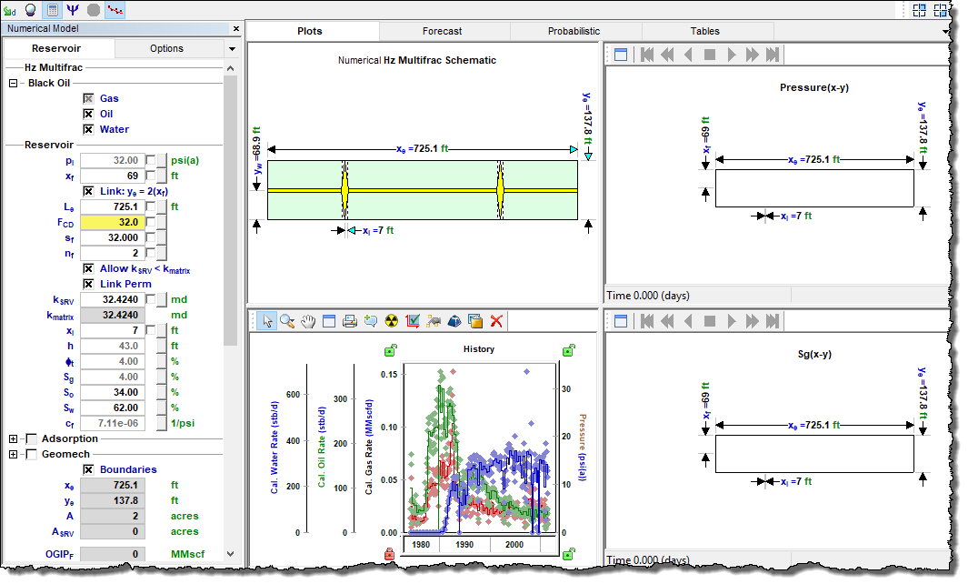
The numerical model has been modified from Harmony to significantly reduce computation time, so that it is almost as fast as an analytical model. For more information, see numerical model theory.

Note:

This analysis works with your Harmony Reservoir™ license.

Before you start using the numerical model, make sure that all required information is added to the Harmony Enterprise project. Well production data (rates and sandface pressures) should be populated in the Production editor, and reservoir and fluid properties should be specified in the Properties editor. When you create a new numerical model, reservoir properties are automatically applied.

We recommend that you perform an analysis prior to using the numerical model as a starting point for other model parameters. For example, for conventional wells, a flowing material balance (FMB) gives an estimate for original fluid in-place, and the use of a typecurve analysis provides insight about permeability, skin, reservoir shape / size, and fracture properties. For unconventional wells, an unconventional reservoir analysis can be used to estimate permeability, fracture length, apparent conductivity, and the size of the stimulated reservoir volume.

You can history match your data using two methods (automatic parameter estimation (APE) and synthesize), but there are important differences.
APE — you can select one or more parameters, and the numerical model keeps the other parameters constant while the parameters being varied are adjusted to reduce the average error between the production history and the model's results.
Synthesize — does not change parameters, but rather all historical data and the parameters in the table are used to run the model. The "match" is what is displayed after the model has been run.
For more information, see the primary toolbar where both of these icons are described.

Numerical Model pane

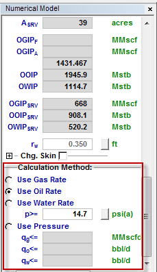
In the Numerical Model pane, enter the required parameters, and select your calculation method. You can use the rates of any of the fluids displayed in the model to calculate rates for the remaining fluids, and the sandface flowing pressure. Or, you can use the sandface flowing pressure to calculate rates for all the fluids displayed in the model.

Hybrid Model pane

For information on the numerical model's options, see advanced options.

Important parameter limits

Note that these parameter limits apply:

k_x, k_y > 0
skin: -8 ≤ s < 200
s_lim (located within the Chg Skin section): -8 ≤ s_lim < 200
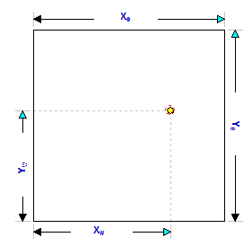
MinXY / 2 < X_w < X_e - MinXY / 2
MinXY / 2 <Y_w< Y_e - MinXY / 2

Fluid type selection

With numerical worksheets, you can select these fluid types based on the fluid behavior you want to simulate:

Gas + Immobile Water — used to create a single-phase model. Only gas flow is modeled in this case; water is considered immobile. If you create a Gas+Immobile Water numerical model for a liquid-rich gas well, the model is calculated in terms of recombined gas (see recombination).
Black Oil — accounts for gas dissolved in liquid, but does not account for liquid vaporized in gas; therefore, you should not create a Black Oil model for liquid-rich gas wells. Oil and water phases can be turned off within the model.
Gas Condensate — used to create a multiphase model that accounts for liquid vaporized in gas. This model should only be used for liquid-rich gas wells. Condensate and water phases can be turned off within the model.
Volatile Oil — used to create a multiphase model that accounts for liquid vaporized in gas. The water phase can be turned off within the model.

Model geometry

Harmony Enterprise supports the following:

Vertical — this model contains a vertical well located anywhere within a rectangular-shaped homogeneous reservoir.
Vertical with Fracture — this model contains a hydraulically fractured vertical well located in the center of a rectangular reservoir. The fracture is surrounded by a symmetrical region of higher permeability.
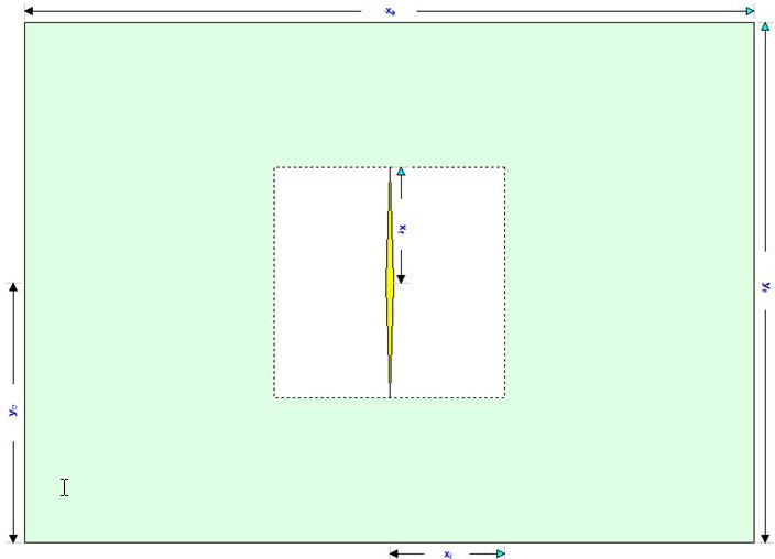
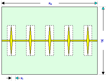
Horizontal Multifrac — this model enables you to specify an enhanced permeability in a region around each fracture. It contains an inactive horizontal well fed by multiple identical, and equally spaced, transverse fractures. The length of the reservoir is defined by the horizontal well. The extent of the enhanced region in the y-direction is defined by the fracture length.
$Horizontal Multifrac model$

Primary toolbar

There are three toolbars: primary, Plots sub-tab, and Forecast sub-tab.

The primary toolbar has the following icons:

Defaults — copies parameters from the Properties editor or other Reservoir worksheets. If you have any analytical gas horizontal multifrac model created for the same well, we recommend that you use it to populate the numerical model's parameters.
Or, if you want to copy only one parameter from an analysis, click the View Defaults and Limits button to the right of the field in the Numerical Model pane.
Note: Parameters copied from the reservoir or another analysis are displayed in a gray font. This indicates that they match the default. You can type new values for any parameter, or change values for some parameters by moving elements of the schematic. Parameters, which do not match the default, will be shown in a black font.
Automatic Parameter Estimation (APE) — while APE is running, selected parameters are automatically varied to minimize the error between the simulated pressure / rate and the actual pressure / rate depending on the calculation method (rate or pressure calculation method — for additional information, see the numerical model pane). The updated simulated pressure / rate is shown on the plots while the calculation is running. While APE is running, the icon appears selected. To stop APE, click the icon again and it no longer appears selected. The model remains at the last parameter set and the history matching finishes calculating for the model. For more information, see using APE (same functionality as with the analytical worksheet).
Important: The purpose of history matching is to get the calculated pressures to reproduce actual pressures as closely as possible by changing the model's parameters. You can vary model parameters manually, or use APE.
AutoCalc — recalculates the history match and forecast automatically each time you change model parameters.
Synthesize — if you do not click the AutoCalc icon, you must click this icon every time you want to recalculate the model.
Stop Synthesize — stops the model's synthesize calculations.
Use Sparse Production Data — opens the Use Sparse Production Data dialog box where you specify the number of timesteps for simulation. This enables you to run simulations with a smaller number of timesteps in order to speed up calculation times. For more information, see sparse data.

You can switch which plots are displayed in the dashboard by clicking the Add an available view icons (to the far right of the other icons on the primary toolbar).

— select a plot to be displayed in the top right corner of your dashboard.
— select a plot to be displayed in the lower right corner of your dashboard.

Sub-tabs

There are three sub-tabs: Plots, Forecast, and Tables.

Plots

This sub-tab displays a schematic and plot from your well data.

Toolbar

This toolbar has the following important icons:

Reset Plot Attributes — resets your plot attributes to default settings.
Picture in Picture — opens the Zoomed View popup where you can get a closeup view of your datasets.
Weight Data Points — used to emphasize matching to specific data points when using APE (for example, the last part of the production). The cursor changes to a spray gun when clicked. Weighted data points are displayed in a brighter color and are given a 100% weighting; unweighted points are given a 10% weighting. (The weighting is displayed when you hover over the data point.)
Copy — copies plot data.
Hide the Toolbar — hides the toolbar. If you want the toolbar displayed, right-click the plot and select Show Toolbar.

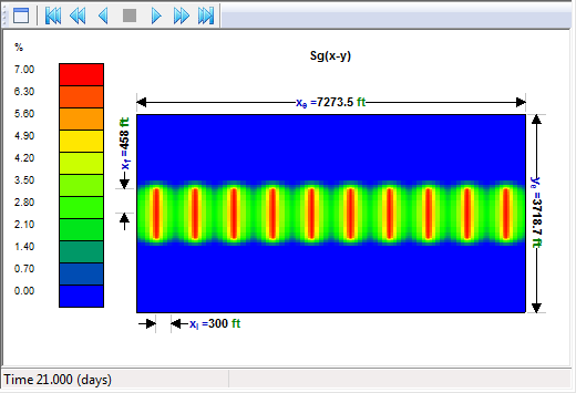
After you click the Synthesize icon ( Synthesize icon ) in the primary toolbar and the calculations are complete, the icons listed below are enabled in your color-shading plots (vertical, vertical fracture, horizontal, horizontal multifrac). With these playback icons, you can see how pressures or saturations change through time. A schematic for your color-shading plot is displayed as long as you specify reservoir dimensions, and the schematic is updated as you change reservoir parameters (for example, X_e, Y_e). A tooltip displays your value and unit, as well as your cursor's x- and y-position within the model as you hover over your color-shading plot.

Skip to Beginning — resets the display to how things were prior to clicking the Synthesize icon.
Step Back One Frame — view calculations in reverse one frame at a time.
Play in Reverse — view calculations in reverse. You can click this icon multiple times to increase the speed of the playback.
Stop — stops the playback process.
Play — view calculations from start-to-finish. You can click this icon multiple times to increase the speed of the playback.
Step Forward One Frame — view calculations one frame at a time.
Skip to End — shows the last calculation.

For information on common plot icons, see plot toolbars.

As the numerical model is calculating results, the color-shading plots update every 100 ms. These intervals are maintained in the steps that are available to play as an animation. When a model calculates very quickly, fewer steps are available, resulting in large jumps for the timesteps displayed.

Forecast

This sub-tab has a toolbar, and displays your forecast: options, constraints, and results.

After the model has been populated and calibrated to the production and pressure data through history matching, production forecasts can be created and compared under a variety of different constraints. This can also be used to create a production forecast for wells with no production history.

Toolbar

This toolbar has the same common icons described in plot toolbars.

Forecast options

The Forecast Options section is where forecast periods are defined according to either durations (for example, months), or dates.

Setting the forecast time method to Duration begins a forecast at a specified start date. Forecast periods are then defined in the forecast table according to a length of time (the default is months). For each forecast period, different operating conditions can be specified.
Setting the forecast time method to Start Date creates a forecast of a specified length of time (the default is months). Forecast periods are then defined in the forecast table according to calendar dates.

Forecast Options

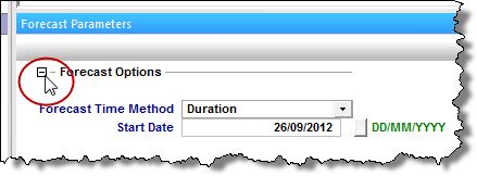
If you select Duration from the Forecast Time Method drop-down menu, the Start Date is automatically populated. (You can change this date later, if needed.)

Forecast Parameters

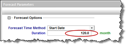
If you select Start Date from the Forecast Time Method drop-down menu, enter a value for Duration (that is, the total length of the forecast).

Duration

Further details about each forecast period are entered in the forecast options table.

Forecast options table

Each row of the table above represents a forecast period. An additional forecast period can be added each time an operational change is encountered (for example, the flowing pressure decreases when a compressor is added). To add a row, use the down arrow when the cursor is in a cell of the last existing row.

The forecast options table has the following sections:

Time — defines the length of each forecast period and each timestep, and has the following columns:
- Step Type — sets the spacing of the timesteps, and can be set to either Arithmetic or Logarithmic. The Arithmetic step type spaces the number of timesteps equally over the total duration of the period, whereas the Logarithmic step type spaces the number of timesteps logarithmically (that is, increased density near the beginning of the forecast).
- Forecast Time Method (Duration / Start Date) — sets the length of the forecast period. If the Forecast Time Method is set to Duration, this column shows Duration. If the Forecast Time Method is set to Start Date, this column show Start Date.
- # of Steps — sets the number of timesteps in the forecast period.
Control — defines how the operating conditions change over the forecast period, and has the following columns:
- Interpolation — can be set to either Step or Ramp. "Step" keeps the control type constant over the forecast period. "Ramp" varies the control type linearly from an initial value to a final value.
- Control Type — sets what is used to calculate the forecast. For the numerical model, the forecast can be run using either flowing pressure, or one of the rates being analyzed.
Sandface Pressure — if the Control Type is set to Pressure, this column is displayed, and it is used to set the flowing pressure for the forecast period. If Interpolation is set to Step, only the initial pressure cell is editable. If Interpolation is set to Ramp, initial pressure and final pressure are selectable.
<Fluid> Rate — if the Control Type is set to a <Fluid> Rate, this column is displayed, and it is used to set the rate for the forecast period. If Interpolation is set to Step, only the initial rate's cell is editable. If Interpolation is set to Ramp, initial rate and final rate are editable.

Forecast constraints

The Forecast Constraints section is where maximum rate conditions and abandonment rate conditions for the forecast can be entered. Available constraints include the following:

p_min — the minimum allowable sandface flowing pressure during the forecast. In order to ensure flowing pressure does not go below this value, rates are adjusted.
(q_g)_max — sets a maximum fluid rate during the forecast. In order to maintain the maximum fluid rate constraint, flowing pressure is adjusted.
(q_g)_ab — sets the abandonment fluid rate for the forecast. When the abandonment rate is reached, the forecast ends.

Forecast results

The Forecast Results section is where the results of the forecast are summarized. Available results depend on the analysis type, and could include the following:

EUR — expected ultimate recovery.
Note: For wells with historical data, EUR is defined as the cumulative of the historical data up to the beginning of the forecast, after which time, the synthetic cumulative calculated from the model is used until the end of the forecast.

RR — remaining recoverable.

Tables

The sub-tab displays your history match (after you use the synthesize or APE functionality) and forecast data (after you populate all the required values in the Forecast tab) in a tabular format.

Note:

The single-phase model (Gas + Immobile Water) is the only model that displays the Blasingame plot on the dashboard. This plot is created using the gas analytical model with identical input parameters. (To generate a Blasingame plot for the horizontal multifrac numerical model, Harmony uses a gas analytical enhanced frac region model. To generate a Blasingame plot for the vertical numerical model, Harmony Enterprise uses a gas analytical vertical model.)

For more information, see tables.