The Economics tab displays the economics for a well, scenario, or group of wells on a monthly basis, and you can run economics for multiple cases with multiple wells. Economics are calculated on a monthly basis by:
- taking the estimated production from decline curve analysis
- multiplying the production volume by the oil, gas, condensate, water, or BOE price that applies to the well at that month
- subtracting fixed and variable expenses
- calculating net revenues for the month
| Note: | Economics works with your Harmony Forecast™ license. |
After clicking Add Case, the Case section opens. Click the inverted chevron icon (![]() ) to open the case section.
) to open the case section.
Case
In this section, you can type a name for your economics scenario and add notes. Only one case can be open at a time.
A case can be added to a single entity or multiple entities.
Case — the title for your economics scenario. You can rename your case by clicking the Case field and typing a new name, or you can leave the default name. However, you cannot have cases with the same name. If you rename a case, its order in the list of cases is automatically resorted alphabetically.
Notes — (optional) click this field to begin typing your notes.
The effective date and duration date are displayed in gray text below the toolbar icons. These dates are automatically taken from the production data you select in the Forecast section. For example, if you have a gas forecast that ends earlier than an oil forecast, the duration date is extended to match the oil forecast's end date for the analysis.
Toolbar
These icons are displayed at the top of the Case section:
![]() Delete Case — removes the currently selected case. If you delete the last case, your settings are reset to the default blank settings (the initial view).
Delete Case — removes the currently selected case. If you delete the last case, your settings are reset to the default blank settings (the initial view).
![]() Copy Case — creates a duplicate of the currently selected case. The name is appended with the word "Copy".
Copy Case — creates a duplicate of the currently selected case. The name is appended with the word "Copy".
![]() Show / Hide Case — toggle between showing or hiding the plot / grid for the currently selected case.
Show / Hide Case — toggle between showing or hiding the plot / grid for the currently selected case.
Discount Rate
The discount rate is a percentage discount, which is applied per year. This adjustment applies to your monthly cash flows received in the future to show its present value.
Type your annual discount rate for your case. The default value is 10%.
Forecast
In this section, up to five fluids can be displayed: oil, gas, condensate, barrel of oil equivalent (BOE), and water.
Your forecast is selectable from the existing decline analyses you have for the currently selected entity.
Select forecast data — select from the drop-down list. If there is an issue with your selection, the Fluid table below displays an error message (for example, invalid forecast, no forecast, etc.).
Note: Forecast volumes are only displayed for the fluids (that is, oil, gas, or BOE) that apply to the currently selected entity, and you can only select one forecast (not one forecast for each fluid).
Price & Revenue
In this section, up to five fluids can be displayed: oil, gas, condensate, BOE, and water.
Type your price, percentage of escalation / year, and your revenue is automatically calculated.
Revenue represents money you have earned before any expenses are accounted for.
![]() Edit Price Deck — opens the Enter Price Decks dialog box. Click this icon to paste values from an existing price deck, or type prices for your fluids. Note that if your price deck has an end date that falls short of the duration date of the forecast for your analysis, the last value in the Price Deck table is used for the remainder of the forecast period. If you paste content with more rows than are automatically displayed in the Price Deck table, note that additional rows are automatically added.
Edit Price Deck — opens the Enter Price Decks dialog box. Click this icon to paste values from an existing price deck, or type prices for your fluids. Note that if your price deck has an end date that falls short of the duration date of the forecast for your analysis, the last value in the Price Deck table is used for the remainder of the forecast period. If you paste content with more rows than are automatically displayed in the Price Deck table, note that additional rows are automatically added.
| Tip: | To decouple your case from a price deck, you need to delete the content in the Enter Price Decks dialog box. Then, you can type a price and percentage of escalation for your fluids. |
Capital Expenses
Capital expenses represent investments that generate benefits for more than one period (for example, drilling, completions, tanks, buildings, etc.).
| Tip: | For upfront costs, leave the Date field blank. These costs are not included in the net present value (NPV) calculation. |
Description — type a name for your capital expense.
Date — select a month from the calendar. Note that you must enter a date between the effective date and duration date for your economic analysis.
Dollar Amount — type a value for your capital expense.
![]() Delete icon — deletes the currently selected capital expense.
Delete icon — deletes the currently selected capital expense.
![]() Add icon — adds a new capital expense item.
Add icon — adds a new capital expense item.
Operating Costs
Operating costs represent expenditures that generate a benefit for the current period (for example, labor, maintenance, water disposal, etc.).
Description — type a name for your operating cost.
Dollar Amount — type a value for your operating cost.
Operating Cost Type — select from the drop-down list (that is, $ / month, $ / year, $ / bbl, $ / Mscf).
![]() Delete icon — deletes the currently selected operating cost.
Delete icon — deletes the currently selected operating cost.
![]() Add icon — adds a new operating cost item.
Add icon — adds a new operating cost item.
From — select a month from the calendar. Note that you must enter a date between the effective date and duration date for your economic analysis.
to — select a month from the calendar. Note that you must enter a date between the effective date and duration date for your economic analysis.
Note: If no dates are selected, by default, the effective date and duration date are used.
Taxes & Royalties
Taxes and royalties are calculated as percentages for the following categories:
Severance Tax — type your percentage. This tax is calculated based on oil & gas earnings before deductions for operating costs, and is also known as the production tax.
Ad Valorem Tax — type your percentage. This "according to the value" tax is calculated based on local taxes (for example, metro district tax, county tax). It is calculated based on revenue less the severance tax.
Royalties — type your percentage. This tax is calculated based on the ongoing right to use certain properties or assets. This tax may be based on a percentage of revenues, or a fixed price per unit sold.
| Note: | Taxes and royalties are calculated for the duration of the forecast, not annually. |
Working Interest
Type your percentage of working interest for revenue and operating costs, which applies for the entire course of the project.
If you want to apply your operating interest to all capital expenses, click this checkbox.
Cumulative Net Cash Flow
This represents a summation of all the values for your case.
Important metrics
These metrics are displayed at the bottom of the plot:
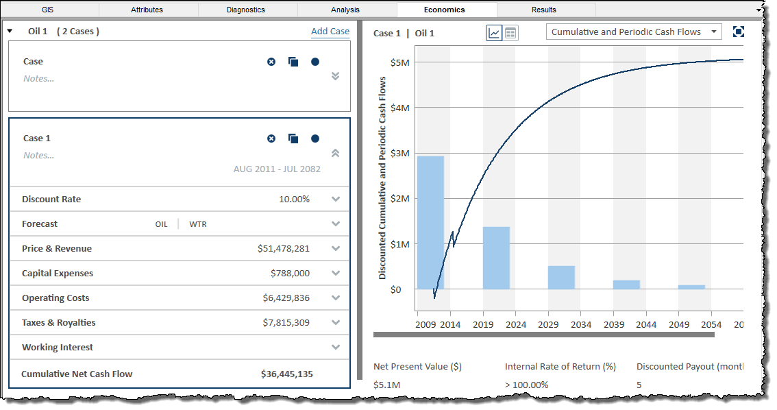
Net Present Value ($) (NPV) — provides the dollar value of a project taking into account the time value of money.
Discounted Payout — the length of time it takes in months to pay back the original investment. If you are running economics on an existing well, the discounted payout is zero.
Internal Rate of Return (IRR) — measures the potential profitability of a project. This metric is a discount rate that measures the percentage of return needed in order for the project to break even (where NPV is equal to zero). IRR is used to evaluate the attractiveness of a project, and is also known as the discounted cash flow rate of return. Generally, if the IRR is a high percentage, this indicates that you have a good project to invest in.
Plot / grid
The cash-flow plot is displayed in the main pane of the Economics window and has the following icons:
![]() Show Plot — displays a plot view for your case. Up to 10 cases can be plotted with cumulative and periodic cash flows. If you plot more than 10 cases, only the cumulative values are displayed. Note that the active case is displayed in bold on the plot.
Show Plot — displays a plot view for your case. Up to 10 cases can be plotted with cumulative and periodic cash flows. If you plot more than 10 cases, only the cumulative values are displayed. Note that the active case is displayed in bold on the plot.
![]() Show Grid — displays a tabular view for your active case, which can be copied and pasted, or exported as a .csv file.
Show Grid — displays a tabular view for your active case, which can be copied and pasted, or exported as a .csv file.
![]() Export to .csv — (only visible when the Show Grid icon is selected) copies your tabular data to a .csv file.
Export to .csv — (only visible when the Show Grid icon is selected) copies your tabular data to a .csv file.
![]() Rescale plot to show all data — (only visible when the Plot icon is selected) automatically fits all your data to the plot.
Rescale plot to show all data — (only visible when the Plot icon is selected) automatically fits all your data to the plot.
The following drop-down list items are only visible when the Plot icon is clicked:
Cumulative and Periodic Cash Flows — displays both the cumulative cash flow and period cash flow on the same plot.
Periodic Series Cash Flows — depending on how you scale the resolution on the x-axis, cash flow is displayed in a bar graph by month, quarter, year, or every five years.
Cumulative Series Cash Flows — displays an aggregate of cash flows in a line graph. The point where the line graph crosses the x-axis is the break-even point.
Y-axis icons
These icons are displayed when you hover your mouse over the y- axis:
 y-axis panning — visible when you hover over the middle of the y-axis, and enables you to pan the axis up and down.
![]() y-axis panning with a lock on the top of the top of the axis — visible when you hover over the lower part of the y-axis, and enables you to pan the axis up and down, while you maintain the top value on the y-axis.
y-axis panning with a lock on the top of the top of the axis — visible when you hover over the lower part of the y-axis, and enables you to pan the axis up and down, while you maintain the top value on the y-axis.
![]() y-axis panning with a lock on the bottom of the axis — visible when you hover over the upper part of the y-axis, and enables you to pan the axis up and down, while you maintain the lower value on the y-axis.
y-axis panning with a lock on the bottom of the axis — visible when you hover over the upper part of the y-axis, and enables you to pan the axis up and down, while you maintain the lower value on the y-axis.
X-axis icons
These icons are displayed when you hover your mouse over the x- axis:
 x-axis panning — visible when you hover over the middle of the x-axis, and enables you to pan the axis left and right.
 x-axis panning with a lock on the right of the axis — visible when you hover over the left-side of the x-axis, and enables you to pan the axis left and right, while you maintain the value on the right.
 x-axis panning with a lock on the left of the axis — visible when you hover over the right-side of the x-axis, and enables you to pan the axis left and right, while you maintain the value on the left.