The following theory is focused on oil as the flowing fluid of interest. The pseudo-pressure referenced is the “oil” pseudo-pressure. A parallel discussion, mutatis mutandis (after the necessary changes have been made), is relevant when gas is the primary fluid of interest.
The Agarwal-Gardner (A-G) flowing material balance (FMB) plot yields the original-oil-in-place as the x-intercept, and the pseudo-productivity index as the y-intercept. The pseudo-productivity index is given by:

The pseudo-productivity index depends on the average reservoir pseudo-pressure, the flowing pseudo-pressure, and the flowing rates of the three producing fluids: oil, gas, and water. The pseudo-productivity index is a parameter that combines Darcy’s law, material balance, and accounts for the variations of fluid and reservoir properties such as: viscosity, formation volume factor, oil-gas-water saturations, geomechanical effects, desorption, etc.
Multiphase FMB uses the rigorous material balance equation to determine the average reservoir pressure, as a function of oil, gas, and water production for specified values of original-oil-gas-water-in-place. Multiphase FMB can account for the presence of water influx, and includes both production and injection rates. In addition, multiphase FMB also takes into account variations of fluid and reservoir properties such as: formation volume factor, oil-gas-water saturation, geomechanical effects, and desorption.
Having determined the oil pseudo-productivity index and the average pseudo-pressure in the FMB analysis, the FMB model uses the pseudo-productivity index and material balance equations in reverse, as follows:
1. Using the pseudo-productivity index:
- Oil Rate — uses the measured flowing pressure to calculate a synthetic oil rate, and compares the synthetic and measured oil rates. Modifies the productivity index and the original-oil-in-place, N, until an acceptable history-match of the oil rates is obtained.
- Flowing Pressure — uses the measured oil rate to calculate a flowing pressure, and compares the synthetic and measured flowing pressures. Modifies the productivity index and the original-oil-in-place, N, until an acceptable history-match of the flowing pressures is obtained.
- Average Pressure — uses the measured flowing pressure and the flowing oil rate to calculate a synthetic average reservoir pressure. Modifies the productivity index and the original-oil-in-place, N, until an acceptable history-match of the average pressure with 2a (see below) is obtained.
2. Using the material balance equation:
- Average Pressure — uses the measured flowing pressure and the flowing oil rate to calculate a synthetic average reservoir pressure. Modifies the productivity index and the original-oil-in-place, N, until an acceptable history-match of the average pressure with 1c (see above) is obtained.
Novelty of the FMB model
Historically, the FMB analysis is based on the A-G analysis (Agarwal et al. 1999). An example of an A-G FMB plot is shown in Figure FMB-Model-1a and FMB-Model-2a. This example is a multiphase gas well, but the FMB model applies to multiphase oil wells as well.
Figure FMB-Model-1a and FMB-Model-2a are plots of different analyses of the same data. Both analyses appear reasonable, but they give significantly different answers. It is obvious that for this dataset, the analysis' straight line can be placed in many locations, and that the corresponding original-gas-in-place values are non-unique over a wide range. Up until recently, there was no way out of this dilemma.

The FMB model solves this problem by creating a history-match of the flowing pressures, or the flow rates.
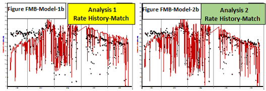
Figure FMB-Model-1b shows the rate history-match corresponding to Analysis 1. Clearly, this history-match is unacceptable. On the other hand, Figure FMB-Model-2b shows the rate history-match corresponding to Analysis 2. Clearly, this is an excellent history-match and confirms that the original-oil-in-place determined from Analysis 2 is consistent with the data, whereas that of Analysis 1 is inconsistent.
Similarly, Figure 1c and 2c are history-matches of the flowing pressures and confirm that Analysis 1 is incorrect, and that Analysis 2 is correct.

In addition to the rate history-match and the flowing pressures history-match, the FMB model can generate the average pressure within the drainage area of a well. This is shown in Figure FMB-Model-1d and FMB-Model-2d. The average reservoir pressure can be generated in two ways: from the productivity index (PI) and from the material balance (MB). When these two methods are congruent, the analysis is correct, as shown in Figure FMB-Model 2d. The utility of this plot is discussed further in reservoir group identification.

The conclusion for this example, is that the original-oil-in-place for this well is 90 BCF. This conclusion would not have been possible without the FMB model.
Reservoir group identification
The objective for using the Reservoir Group Identification plot is to identify which wells are in the same reservoir, and which wells are in separate reservoirs. If there are several wells producing from the same reservoir under stable conditions, they establish their own drainage areas, approximately in proportion to their flow rates. These drainage areas vary in shape and size, and depend in part on the flow rates. If the well's flow rates change, the no-flow boundaries between the wells move, and each well’s drainage area changes correspondingly, until all the drainage areas have the same average pressure within them.
The phenomenon that, under stable flowing conditions, wells in the same reservoir have a common average pressure within their drainage areas as a function of time, provides a diagnostic to identify if two wells are in the same reservoir, or in different reservoirs.
Using the FMB model, the average pressure within the drainage area can be determined by selecting Average Pressure — see Figure FMB-Model-2d above. For each well, determine the correct average pressures (FMB Model Pressure-PI) as shown in Figure 2d. Compare these average pressures in the Comparison plot, as a function of time. If they follow the same trend, they most-likely belong to the same reservoir — (see Wells A and B in Figure 3), and if they have different trends, they most-likely belong to separate reservoirs — (see Well C in Figure 3).
