You are here:

Multiphase flowing material balance (FMB) theory

There is significant research in the field of multiphase FMB, and rate-transient analysis in general, that is ongoing at the University of Calgary, under the direction of Dr. Chris Clarkson. This research has been supported by industry sponsors of the Clarkson-led Tight Oil Consortium, and by NSERC CRD grants held by Clarkson. This partial list of publications attests to the interest, effort, and success of his team in this field. All the methods have a certain number of assumptions and approximations, and are therefore not exact analytical solutions for all flow conditions. For example, they are not meant to be applicable to “transient flow”, but they are intended for analyzing boundary-dominated flow. Our (IHS Markit) development of Multiphase FMB, implemented in Harmony Enterprise version 2018.1 builds on the work of Dr. Clarkson’s team and extends it. Most of the studies define one two-phase pseudo-pressure for oil, and one for gas. Some define a total pseudo-pressure that combines all three phases.

There are two major components to the FMB methodology: defining an appropriate pseudo-pressure and an appropriate pseudo-time. Sometimes, as in the current implementation, pseudo-time is not visible explicitly, but is couched in expressions that combine the average pseudo-pressure and cumulative production.

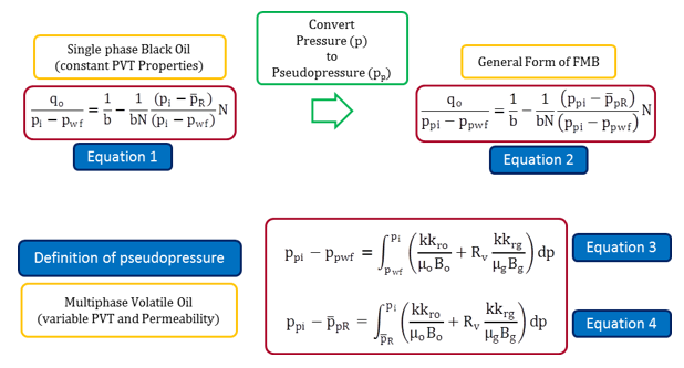
Multiphase FMB parallels the single-phase methodology. In simple terms, single-phase FMB was derived for oil (in terms of pressure). Multiphase FMB uses the same format of equations, but replaces pressure by a pseudo-pressure that accounts for the variations in pressure, volume, and temperature (PVT) properties, saturation changes, relative permeability, and individual flowing phases.

As an introduction, a simplified version of the single-phase FMB formulation is presented below:

(Boundary-dominated flow) fundamental flow equation:

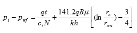
Can be simplified to:

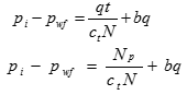
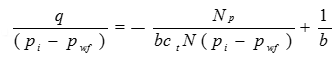
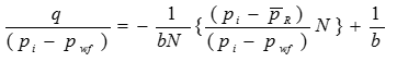
Rearranging — divide by b and by (p_i - p_wf):

Material balance equation:

Combining these two equations:

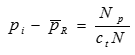
Multiplying top and bottom by N:

This is the FMB equation that is represented in the Agarwal-Gardner (A-G) plot: Plotting the left-side against {…} results in an x-intercept of N (original-oil-in-place), and a y-intercept of 1/b (Productivity Index).

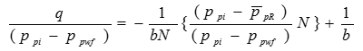
Multiphase FMB equation

The multiphase FMB analysis is structured in a format similar to the above equation, but pressure is replaced by an appropriately defined multiphase pseudo-pressure.

The discussion below is focused on oil as the flowing fluid of interest. The pseudo-pressure defined below is the “oil” pseudo-pressure. A parallel discussion, mutatis mutandis (after the necessary changes have been made), is relevant when gas is the primary fluid of interest.

The “oil” pseudo-pressure defined below accounts for:

multiphase flow — oil, gas, and water, for both production and injection
fluid property variations with pressure
saturation changes in the reservoir caused by production or injection
geomechanical effects, desorption, water influx.

In evaluating the above equations, the following considerations apply:

i: k_rg and k_ro are functions of saturation (not pressure). In order to evaluate the pseudo-pressure integral, the k_rg and k_ro functions have to be expressed in terms of pressure (not saturation). Therefore, we need to have a relationship between saturation and pressure. However, saturations depend on production. Consequently, multiphase pseudo-pressure can only be evaluated after the production rates are known. This is in contrast to single-phase pseudo-pressure, where the pseudo-pressure can be evaluated independently from production.

ii: At any point in time, the flow rates of gas, oil, water, and the flowing pressures are known from measurement. The average reservoir pressure is obtained from material balance equations.

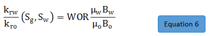
iii: At any point in time, using the production data, the k_rg / k_ro ratios are determined from:

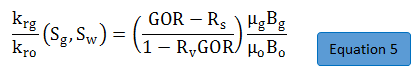
And the k_rw / k_ro ratios are obtained from:

iv: The relative permeability curves are reformulated in terms of k_rg / k_ro ratios versus saturations. The k_rg / k_ro ratios will be a single curve for two-phase (gas / oil) flow, but become a surface, when water production is included.

v: From the permeability ratios obtained from production data (see step iii) and the relative permeability curves (see step iv), the saturations are obtained for every point in time, and the corresponding pseudo-pressure is evaluated, using Equations 3 and 4.

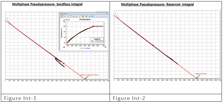
vi: The calculation of pseudo-pressure involves the evaluation of an integral. In the literature, there are two ways of doing this: a) using the Sandface Integral, or b) using the Reservoir Integral. The more rigorous of the two is the Reservoir Integral, and that is what is used in the current implementation of Harmony Enterprise. It recognizes that the saturations change, not only through time, but also with location in the reservoir. This makes the pseudo-pressure calculations complex, cumbersome, and iterative. At every point in time, they consist of a stepwise integration from to , and from to .
As a result, because analysis lines are dynamically calculating the pseudo-pressures, the line movement can be slow, when there is a large number of data points. Figure Int-1 and Int-2 below demonstrate that the Reservoir Integral is more effective in straightening out the multiphase data than the Sandface Integral.

vii: On the basis of Equation 2, an FMB (A-G) analysis is created by plotting versus .
Since the Oil-In-Place, N, is not known, the solution is iterative. The value of N is modified until the data forms a straight line. This is illustrated in Figure FMB-1 and FMB-2.

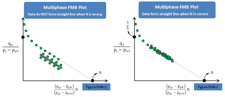
The x-intercept is the desired value of N. The y-intercept (1/b) is the (pseudo) Productivity Index, which is defined as:

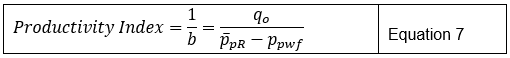
viii: The productivity index varies during transient flow, but becomes constant during boundary-dominated flow. Because the pseudo-productivity index is defined in terms of pseudo-pressures, variations in saturation and relative permeabilities are accounted for (albeit in an approximate manner). As a result, the pseudo-productivity index becomes a constant (dependent only on reservoir shape, size, initial permeability, initial saturations, and well completion, which are all considered to be constant).

ix: For oil wells producing below the bubble point or producing water, the results of the multiphase FMB can be significantly different from a single-phase oil analysis.

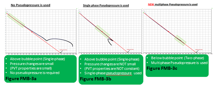
x: For oil wells producing at a flowing pressure above the bubble point, the gas produced is purely solution gas, and flow in the reservoir is actually single phase. In this situation, the traditional single phase (using “pressure” for analysis) can yield the correct value of N at the beginning (when PVT properties are still relatively constant) — see Figure FMB-3a. When PVT properties change (while still in single-phase flow), a single-phase pseudo-pressure can be defined, and this straightens the data — see Figure FMB-3b. When pressures go below the bubble point, multiphase flow occurs and the multiphase pseudo-pressure defined above must be used to straighten the data, and obtain the correct value of N. This is demonstrated in Figure FMB-3c.

Important considerations

The multiphase FMB equations are developed for boundary-dominated flow, and like most reservoir engineering equations, involve simplifying assumptions. Since the multiphase FMB model has only recently been implemented, the effect of these assumptions has not been extensively evaluated, and the results must be used with caution until they have been verified in everyday production situations. Some of the issues that need to be validated through use and independent confirmation of results are discussed below:

In some of the following situations, anomalies in the behavior of the data (even synthetic data) have been observed:

When the bubble / dew-point pressure is crossed while production is still in transient flow. However, it is expected that the data catches up to the correct trend as production continues.
Selecting Liquid-Rich Gas in the PVT Properties section. This option is sensitive to any inconsistencies inherent in the PVT properties.
The Z** used in the flowing P/Z** calculation does not account for condensate and water production. Therefore, for rich-gas condensate reservoirs and cases with significant water production, the flowing P/Z** plot may not line up with the analysis line. However, the analysis is correct: the A-G straight line points to the correct Original-Gas-in-Place, and the model's verified gas flow rates and flowing pressures are correct. The only problem is that the P/Z** plot does not match, and this mismatch is not indicative of an incorrect analysis. Rather it indicates that the Z** is not accounting for the liquid production.
In some cases, a minimal adjustment of the relative permeability exponents (for example, changing n_g from 1.5 to 2) does improve the match between the data and the analysis.
When analyzing multiphase production data in FMB, it is possible to generate an incorrect straight-line trend by increasing the volume in place. The recommended procedure is to select the minimum value of original-oil-in-place, which results in an A-G Analysis straight line. This issue becomes more critical when analyzing data that is still in transient flow, especially when the bubble / dew-point pressures are hit before the boundary-dominated flow is reached. An example of incorrect and correct interpretation is shown below (see item h).
Since multiphase FMB takes into account the production rate of all phases that are entered in the Production editor, the often poorly measured or misreported water production rates might result in a more scattered FMB plot. In some jurisdictions, the condensate is inconsistently reported, sometimes as condensate production, sometimes as oil production, and sometimes as part of the (recombined) gas. These issues can be evaluated by removing these poorly reported rates from the Production editor.
In analyzing the multiphase flow in the unconventional reservoir model (URM), moving the end-of-linear flow line in the square-root time plot, may cause the data to move (even when pseudo-time has not been selected). The reason for this is that by changing the end-of-linear flow line, the reservoir size is changing. Therefore, the average pressure, will correspond to a different saturation distribution, and as a result, has different pseudo-pressure calculations. For a large reservoir volume, where changes in the saturation profile are not as important as for a smaller reservoir volume (or for single-phase flow), moving the end-of-linear flow line has an insignificant effect on the data.
Since FMB equations are focused on boundary-dominated flow, caution has to be exercised during transient flow. For single-phase flow, the FMB has been used to reliably estimate the “contacted” volume. However, for multiphase flow, it may not be reliable for this purpose, and may give significantly misleading results. Moreover, the effect of flow geometry has not been completely studied. Two examples that illustrate some problems with Linear and Transient Flow are shown below:

Publications

1. Behmanesh, H., Hamdi, H. and Clarkson, C. R. 2015. Production Data Analysis of Liquid Rich Shale Gas Condensate Reservoirs. Journal of Natural Gas Science and Engineering 22: 22–34. 10.1016/ jngse.2014.11.005.

2. Behmanesh, H., 2016, Rate−Transient Analysis of Tight Gas Condensate and Black Oil Wells Exhibiting Two−phase Flow, Ph.D. thesis, University of Calgary.

3. Behmanesh, H., Hamdi, H., Clarkson, C.R. 2017. Production data analysis of gas condensate reservoirs using two−phase viscosity and two−phase compressibility, Journal of Natural Gas Science & Engineering, doi: 10.1016/j.jngse.2017.07.035.

4. Behmanesh, H., Mattar, L., Thompson, J. M., Anderson D. M., Nakaska, D. W. and Clarkson, C. R. 2018. Treatment of Rate-Transient Analysis During Boundary-Dominated Flow. SPE Journal, SPE 189967-PA doi:10.2118/189967-PA

5. Camacho−v, R. G., and Raghavan R. 1989. Performance of wells in solution−gas−drive reservoirs. SPE Form Eval 4.(4) 611−620. SPE−16745−PA. DOI: 10.2118/16745−PA.

6. Heidari, M., Behmanesh, H., and Clarkson, C. R. 2013. Multi−Well Gas Reservoirs Production Data Analysis. Presented at the SPE Unconventional Resources Conference Canada, Calgary, 5–7 November. SPE−167159−MS. https://doi.org/10.2118/167159−MS.

7. Heidari, M., Behmanesh, H. and Clarkson, C. R. 2014. New Semi−Analytical Method for Analyzing Production Data from Constant Flowing Pressure Wells in Gas Condensate Reservoirs during Boundary−Dominated Flow. Paper SPE 169515 presented at the SPE Western North American and Rocky Mountain Joint Regional Meeting, Denver, Colorado, 16−18 April. DOI: 10.2118/169515−MS.

8. Jones, J. R., & Raghavan, R. (1988, September 1). Interpretation of Flowing Well Response in Gas-Condensate Wells (includes associated papers 19014 and 19216). Society of Petroleum Engineers. doi:10.2118/14204-PA

9. Raghavan, R. (1976, August 1). Well Test Analysis: Wells Producing by Solution Gas Drive. Society of Petroleum Engineers. doi:10.2118/5588-PA.

10. Shahamat, M. S., & Clarkson, C. R. 2017. Multi−Well, Multi−Phase Flowing Material Balance. Paper SPE 185052 prepared for Presentation at the SPE Reservoir Evaluation & Engineering – Formation Evaluation, SPE 185052-PA doi:10.2118/185052-PA.