Overview
Material balance analysis is an interpretation method used to determine original fluids-in-place (OFIP) based on production and static pressure data. The general material balance equation relates the original oil, gas, and water in the reservoir to production volumes and current pressure conditions / fluid properties. The material balance equations considered assume tank-type behavior at any given datum depth — the reservoir is considered to have the same pressure and fluid properties at any location in the reservoir. This assumption is quite reasonable provided that quality production and static pressure measurements are obtained.
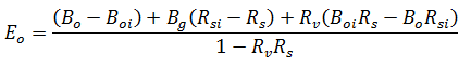
Consider the case of the depletion of the reservoir shown below. At a given time after the production of fluids from the reservoir has commenced, the pressure drops from its initial reservoir pressure pi, to some average reservoir pressure, p. Using the law of mass balance, during the pressure drop (Dp), the expansion of the fluids left over in the reservoir must be equal to the volume of fluids produced from the reservoir.

The simplest way to visualize material balance is that if the measured surface volume of oil, gas, and water were returned to a reservoir at the reduced pressure, it must fit exactly into the volume of the total fluid expansion, plus the fluid influx.
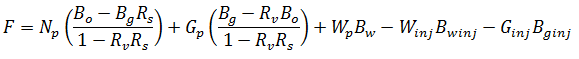
The general form of the equation can be described as net withdrawal (withdrawal - injection) = expansion of the hydrocarbon fluids in the system + cumulative water influx. This is shown in the equation below.

Each term in the equation can be grouped based on the part of the system it represents. The table below shows the terms and a simplified version of the general equation based on the terms.
Summary of terms in the material balance equation
| Term | Description |
|---|---|
|
|
Simplified general equation. |
|
|
Volume of withdrawal (production and injection) at reservoir conditions is determined by the oil, water, and gas produced at the surface. |
|
|
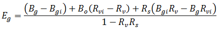
Total expansion. |
|
|
If the oil column is initially at the bubble point, reducing the pressure results in the release of gas and the shrinkage of oil. The remaining oil consists of oil, and the remaining gas still dissolved at the reduced pressure. |
|
|
Gas expansion factor. For example, as the reservoir depletes, the gas cap expands into the reservoir volume previously occupied by oil. |
|
|
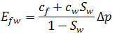
Even though water has low compressibility, the volume of connate water in the system is usually large enough to be significant. The water expands to fill the emptying pore spaces as the reservoir depletes. As the reservoir is produced, the pressure declines and the entire reservoir pore volume is reduced due to compaction. The change in volume expels an equal volume of fluid as production, and is therefore additive in the expansion terms. |
|
|
Ratio of gas cap to original oil in place. A gas cap also implies that the initial pressure in the oil column must be equal to the bubble point pressure. |
|
|
If the reservoir is connected to an active aquifer, then once the pressure drop is communicated throughout the reservoir, the water encroaches into the reservoir resulting in a net water influx. |


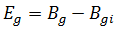


Not all terms are used at any one time, but the purpose of a complete equation is to provide a basis from which to analyze many types of reservoirs: gas expansion, solution gas drive, gas cap drive, water drive, etc. Terms that are not needed for a particular reservoir type cancel out of the equation. For example, when there is no gas cap originally present, the G and Bgi terms are zero.
Application of material balance
Material balance is an important concept in reservoir engineering because it is a performance-based tool used to establish the original volume of hydrocarbons-in-place in a reservoir that typically contains many wells. Additionally, the process of matching pressure-based depletion trends between wells gives the reservoir engineer the ability to create a performance-based view of the connected pore volume in the reservoir. Consequently, it is important that:
1. All fluids taken from, or injected into the reservoir be measured accurately.
2. Pressure, volume, and temperature characteristics (PVT properties) be measured and validated. Subsurface samples from several properly conditioned wells are preferred.
3. At least one static pressure from each well prior to production, and several after production has commenced, are required to achieve good results.
The establishment of original-in-place fluid volumes and connected pore volume are critical to the development of ongoing depletion plans, especially where secondary or tertiary recovery methods are being considered.
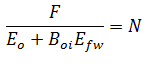
Gas material balance
Gas material balance is a simplified version of the general material balance equation. When the general equation is reduced to its simplest form containing only gas terms, it appears as shown below:
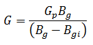
In this equation, it is assumed that gas expansion is the only driving force causing production. This form is commonly used because the expansion of gas often dominates over the expansion of oil, water, and rock. Bg is the ratio of gas volume at reservoir conditions to gas volume at standard conditions. This is expanded using the real gas law.
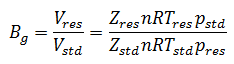
The reservoir temperature is considered to remain constant. The compressibility factor (Z) for standard conditions is assumed to be 1. The number of moles of gas do not change from reservoir to surface. Standard temperature and pressure are known constants. When Bg is replaced and the constants are canceled out, the gas material balance equation then simplifies to:
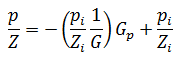
When plotted on a graph of p/Z versus cumulative production, the equation can be analyzed as a linear relationship. Several measurements of static pressure and the corresponding cumulative productions can be used to determine the x-intercept of the plot - the original gas-in-place (OGIP), shown as G in the equation.

Advanced gas material balance
For a volumetric gas reservoir, gas expansion (the most significant source of energy) dominates depletion behavior; and the general gas material balance equation is a very simple, yet powerful tool for interpretation. However, in cases where other sources of energy are significant enough to cause deviation from the linear behavior of a p/Z plot, a more sophisticated tool is required. For this, a more advanced form of the material balance equation has been developed, and the standard p/Z plot is modified to maintain a linear trend with the simplicity of interpretation.
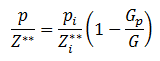
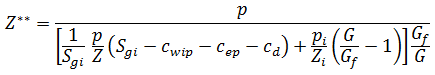
In his work on CBM, King (1993) introduced p/Z* to replace p/Z. By modifying Z, parameters to incorporate the effects of adsorbed gas were incorporated, so the total gas-in-place is interpreted, rather than just the free gas-in-place; and a straight line analysis technique is still used. This concept has been extended to additional reservoir types with Fekete's p/Z** method (Moghadam et al. 2009).
The reservoir types considered in the advanced material balance equation are: overpressured reservoirs, water-drive reservoirs, and connected reservoirs. The total Z** equation is shown below with the modified material balance equation.
Overpressured reservoir
At typical reservoir conditions, gas compressibility is orders of magnitude greater than that of the formation rock or residual fluids. In reservoirs at high initial pressures the gas compressibility is much lower, in the same order of magnitude as the formation. A typical example of this is an overpressured reservoir, which is a reservoir at a higher pressure than the hydrostatic column of water at that depth — in other words, a higher than expected initial pressure given the depth. In this situation, ignoring the formation and residual fluid compressibility results in over-prediction of the original gas-in-place. The initial depletion shows the effects of both depletion and reservoir compaction, and the slope of a p/Z plot is shallower. Once the pressure is much lower than the initial pressure, gas expansion is dominant and a steeper slope is observed on the p/Z plot. When matching on the shallower slope of this bow-shaped trend, all later pressure data is lower than the analysis line, and the estimated original gas-in-place is higher than the true original gas-in-place. The plot below shows an overpressured reservoir matched on the initial data, and the analysis line of the advance material balance method.

Based on the definition of compressibility, the following equation represents the total effect of formation and residual fluid compressibility:
The approximate form of this equation, found by considering compressibility for oil, water, and the formation as constant; and ex as 1 + x, is:
In order to use this compressibility in the material balance equation, the change in pore volume is taken relative to the initial pore volume. The rigorous and approximate forms are shown below.
Rigorous form:

Approximate form:

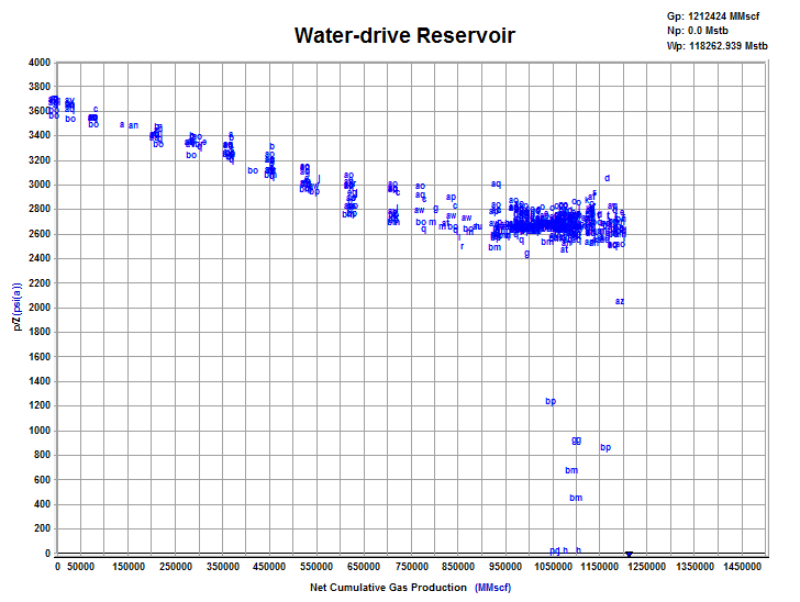
Water-drive reservoir
Some gas reservoirs may be connected to aquifers that provide pressure support to the gas reservoir as it is depleted. In this case, the pressure decrease in the gas reservoir is balanced by water encroaching into the reservoir. As this happens, the pore volume of gas is decreasing and the average reservoir pressure is maintained. Often this reservoir shows a flat pressure trend after some depletion. An example of this behavior on a p/Z plot is shown below.
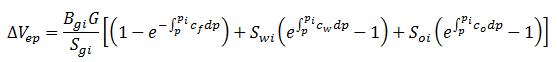
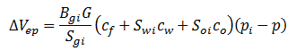
The change in reservoir volume due to net encroached water can be determined from the following equation:

To use this in the material balance, the change in pore volume is taken relative to the initial pore volume, shown below.

When dealing with this equation, the major unknown value to be determined is water encroachment from the aquifer (We). Two aquifer models are provided to determine net encroached water: Schilthuis Steady-State Model and Fetkovich Model.
Schilthuis steady-state model
This is the simplest aquifer model and assumes the rate of water influx is proportional to pressure drawdown. In this model it is assumed that the aquifer volume is much larger than the gas reservoir and remains at the initial pressure.

Using this model, the only parameter to solve for is the transfer coefficient (J).
Fetkovich
In the Fetkovich aquifer, the aquifer is assumed to be in pseudo-steady state and depleted according to the material balance equation. In this model, both the aquifer volume and transfer coefficient must be determined. The equations are shown below.


While the transfer coefficient is defined, the required inputs to calculate the transfer coefficient are often not known. More commonly the transfer coefficient is determined as part of matching the p/Z plot.
Connected reservoir
Another scenario which appears as pressure support on the p/Z plot is the connected reservoir model. The generic description is that two gas reservoirs are connected, described by a transfer coefficient between them, and gas feeds from one tank to the other as one of the tanks is depleted. This can be observed with two gas reservoirs with some communication, two zones in a reservoir with different permeability, or some barrier between them, or even another way of considering the situation of free and adsorbed gas in a reservoir. Because both water-drive and connected reservoirs show pressure support, it can be easy to mistake which model should be used. In a connected reservoir, the influx into the main reservoir is gas, as compared to an influx of water in water-drive. So the pressure support is accompanied by more gas in the reservoir, rather than a shrinking reservoir as in water-drive. Typically if the initial p/Z trend points to an original gas-in-place smaller than the cumulative production, a connected reservoir is the appropriate model to use.

For a connected reservoir, the material balance equation is written as shown below to account for gas influx.
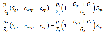
This can be converted into a dimensionless term similar to the terms describing relative change in pore volume (cwip, cep, and cd) for other models, as shown below.

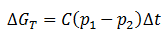
Similar to the water-drive model, the influx of gas from the second reservoir (GT) is likely not a known value, and therefore it must be determined based on the size of the connected reservoir, and the transfer coefficient between the reservoirs. The equation for gas influx is shown below.
Oil material balance
As seen in the general material balance equation, there are many unknowns, and as a result, finding an exact or unique solution can be difficult. However, using other techniques to help determine some variables (for example, m or original gas-in-place from volumetrics or seismic), the equation can be simplified to yield a more useful answer. Various plots are available to conduct an oil material balance rather than calculating an answer from individual measurements of reservoir pressure.
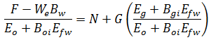
Havlena-Odeh (all reservoir types)
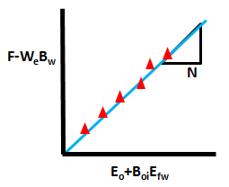
Similar to the interpretation of gas material balance, oil material balance uses plotting techniques. However, unlike the equation for single-phase gas expansion, the standard form of the material balance equation for oil reservoirs does not easily yield a linear relationship. The equation can be organized to show linear behavior. Based on the rearrangement below, the large combinations of terms are used as x and y, while G is the slope, and N is the intercept. This of course implies that water influx term for each data point is a known value, or the simpler scenario that there is no water influx. Additionally, if the water influx is neglected in calculating the terms, the result is non-linear behavior on the plot. This can be a diagnostic to determine the presence of water drive. In practice, the scatter in the data may be great enough, and the signature of water drive subtle enough that deviation from linear behavior on the Havlena-Odeh plot may go unnoticed.
An example of the plot is shown below. The scatter shown in the data points demonstrates the difficulty in determining trends in the reservoir behavior.

- Movement around a — moves the y-intercept. Changes N and keeps G (OGIPf) constant.
- Movement around b — rotates the line around the pivot point. Changes N and G at the same time.
- Movement around c — rotates the line around the y-intercept. Changes G and keeps N constant.
The slope of the line is G and the y-intercept is N. This plot provides a solution to G and N simultaneously. Either G or N can be manually adjusted to achieve the best answer. Care should be taken when using this plot as slight errors in pressure measurements can drastically affect results. The data is more spread out in a cloud-like formation when errors are present in PVT or pressure data.
| Note: | "Scaling" applied to the plot can interfere with the appearance of a trend. Use your judgment when using this analysis. |
This method works for most reservoir types. In the case of an undersaturated reservoir (above bubble point), the Eg + Bgi * Efw term is zero, and this plot is not as useful. The standard Havlena-Odeh plot can be substituted for one that excludes free gas terms.
Havlena-Odeh diagnostics: F vs. Et (no initial gas cap)
If the reservoir to be analyzed has no initial free gas, the free gas terms of the equation can be eliminated. This equation is now much simpler to linearize. In the equation shown below, the total expansion term is split into the oil and water / formation expansion terms. Once again, the inclusion of water influx is such that it is assumed to be known.
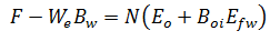
In this form of the equation, N is the slope on a plot of expansion terms versus withdrawal and influx terms. There is no intercept, so the analysis line is typically forced through zero. Similar to the Havlena-Odeh plot that includes gas terms, if water influx is neglected and a non-linear trend results, this can be a diagnostic for observing water-drive effects. An example of the plot is shown below.
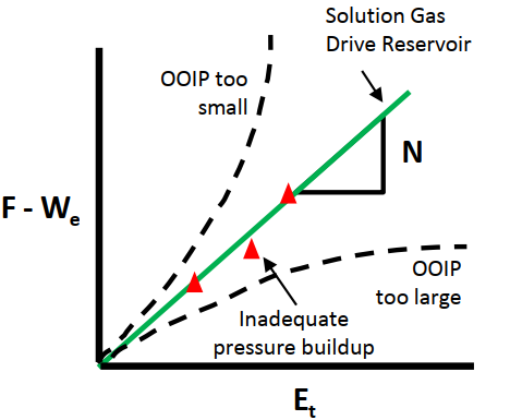
- Linear trend — a linear trend in the data indicates volumetric depletion behavior, or that all external drive mechanisms have been correctly accounted for.
- Upward concave — indicates that the OOIP is too small. Adjusting OOIP will linearize the points along the trend.
- Downward convex — indicates that the OOIP is too large. Adjusting OOIP will linearize the points along the trend.
- Stray point — an inadequate pressure buildup over time may be the reason that a pressure measurement comes in slightly below the predicted trend line. Other reasons may include inaccurate PVT data, or inaccurate production information for that time.
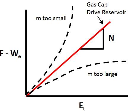
- Linear trend — a linear trend in the data indicates volumetric depletion behavior, or that all external-drive mechanisms have been correctly accounted for. Though it cannot independently determine the oil-in-place volume when a gas cap is present, the F vs. Et plot can assist in confirming the consistency of the proposed solution.
- Upward concave — indicates that the gas cap is too small. Adjusting m or G should linearize the points along the trend.
- Downward convex — indicates that the gas cap is too large. Adjusting m or G should linearize the points along the trend.
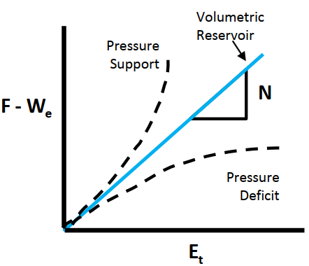
- Linear trend — a linear trend in the data indicates a volumetric expansion reservoir (solution gas or gas cap), provided the OOIP and OGIP are correct. The F vs. Et cannot independently determine the exact reason for pressure support, but it can assist in confirming the consistency of the solution.
- Upward concave — indicates pressure support from unaccounted for water injection, fluid from another reservoir, aquifer, U-tube displacement of a producing reservoir's water leg by a connected reservoir, or the expansion of water.
- Downward convex — indicates a pressure deficit from late-time interference from unaccounted for producing wells, rock compressibility in an over-pressurized reservoir, or inflow that gradually decreases over time due to depletion.
Oil in place diagnostics (N vs. time)
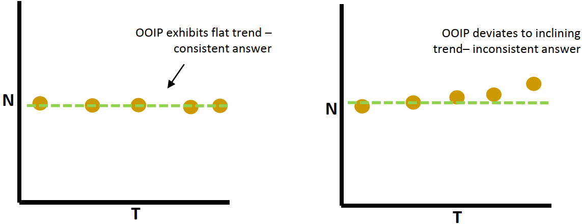
When applying material balance, it is a good practice to examine the validity of the results. The N vs. Time profile provides a useful check as to the consistency of the answer. The value of N is based on the input pressure, production, and PVT data. At each individual reservoir pressure, OOIP is calculated. An inconsistent trend in the OGIP usually indicates that there may be an external-drive mechanism present. This plot is also useful as a diagnostic to determine if the correct reservoir type has been assumed, and to assess the data quality. An inconsistent trend usually indicates that the quality of the pressure measurements are not good, or the definition of the wells in the reservoir should be reviewed. A consistent upward trend indicates that another drive mechanism may be present, whereas a downward trend indicates that not all wells in the reservoir have been included in the analysis. The type of drive mechanism is not evident, only that there is some "other" energy in the system that is not accounted for.
- Flat trend — a flat trend in the N values indicates volumetric depletion behavior, or that all external drive mechanisms have been correctly accounted for.
- Inclining trend — indicates that the reservoir is seeing additional pressure support, either from an aquifer or formation compressibility drive (geomechanical effects). However, the type of external drive mechanism is not distinguishable.
| Note: | This plot is meant to be used as a diagnostic guide to complement the analysis, and we recommend not putting too much emphasis on the interpretation. When there is a low frequency of pressure surveys, a trend may not be visible and this diagnostic plot may be of little value. Scaling" applied to the plot can interfere with the appearance of a trend. Use your judgment when using this analysis. |
Pressure diagnostics: P vs Np
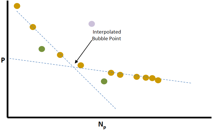
- Inflection — this is where the pressure depletion trend changes. At this point, the first bubble of gas comes out of solution, and the solution-drive-energy mechanism starts to decrease, thus the reservoir depletes at a slower rate.
- Inclining static pressures — indicates the start of gas or water injection.
- Constant pressure — may indicate aquifer support.
- Erroneous pressure data — may indicate that this well is not part of the reservoir.
Pressure vs. time
When applying material balance, it is a good practice to initially examine the pressure depletion profile. Any changes in production during the life of the reservoir should be visible in this plot. For example, the bubble point pressure is visible by a decrease in the pressure decline rate. The start of injection should be seen as an increase in the sandface pressure measurements. Examining the trends prior to the analysis helps give a frame of reference for the analysis. With these trends, you can learn from the diagnostic plots, which can help you understand if the final answers obtained from the analysis make sense.
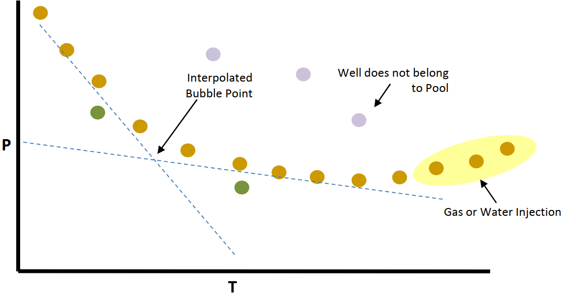
- Inflection — this is where the pressure-depletion trend changes. At this point, the first bubble of gas comes out of solution and the solution-drive-energy mechanism starts to decrease, thus the reservoir depletes at a slower rate.
- Inclining static pressures — indicates the start of gas or water injection.
- Constant pressure — may indicate that boundary-dominated flow has not yet been achieved, or the pressure of aquifer support.
- Erroneous pressure data — may indicate that this well is not part of the reservoir.
| Note: | This plot is meant to complement the analysis plot, and we do not recommend interpretation with pressure on its own. When there is a low frequency of pressure surveys, a trend may not be visible and this plot may be of little value. |
Synthetic reservoir pressure
The pressure match method uses an iterative procedure that uses the values of original oil-in-place, original gas-in-place, and W to calculate the reservoir pressure versus time. The synthetic reservoir pressure is then plotted against the real measured static reservoir pressures and compared. This is by far the most robust and easily understood material balance technique for the following reasons:
1. Pressure and time are easily understood variables, so sensitivity analysis can be conducted relatively easily.
2. Use of time enables the analyst to see directly the impact of:
- Changing withdrawal rates, especially shut-ins on reservoir pressure declines.
- Injection operations on pressure response.
- Water drive and connected reservoirs on reservoir depletion, especially since these are both cumulative withdrawal and time-based processes.
3. A relatively simple, iterative process is used to achieve a unique solution wherein:
- Start with the simplest solution (oil and/or gas depletion only) and then proceed to more complex models only if demonstrated to be required.
- Employ a left-to-right matching technique (early-time to late-time), wherein initial reservoir pressure is matched first, followed by early-time depletion response, and then late-time responses. Since water drive and connected reservoir models are cumulative withdrawals and time-based, their responses are minimal at early-times and maximized at late-times.
Consistent and inconsistent history matches are shown below:

- Good match — the combination of G, N, and We has provided a valid solution to the material balance equation. Note that other combinations of values may exist as the solution is usually non-unique.
- Incorrect / inaccurate PVT data — results in a bad match. This causes problems early on when pressure depletion is low, and results in the oil & gas expansion terms having a large error.
- Outlier production / pressure points — water and solution gas may not be accounted for correctly. Also, outliers or erroneous pressure points may be incorrectly included in the analysis.
- Incorrect pressure data — in low permeability reservoirs, the well may not have been shut-in long enough to obtain a stabilized pressure, so pressure measurements could be on the low side.
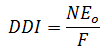
Drive indices
Drive indices for oil reservoirs indicate the relative magnitude of the various energy sources acting in the reservoir. A simple description of a drive index is the ratio of a particular expansion term to the net withdrawal (hydrocarbon voidage). These drive indices are cumulative and change as the reservoir is produced. A plot of drive indices and the details of specific drive indices are shown below.

Summary
| Drive Index | Description |
|---|---|
|
Depletion drive index |

|
Segregation (gas cap) drive index |

|
Water drive index |

|
Formation and connate water compressibility index |
If the drive indices do not sum to unity (or very close to 1), the correct solution to the material balance has not been obtained.
Diagnostics

- Sums to approx 1 — high probability that the correct solution to the material balance equation has been obtained.
- Does not sum to 1 — the correct solution has not been obtained. If the summed drive indices are consistently greater than or less than unity, or show a consistent increasing or decreasing trend, this indicates that the correct solution has not been found. Possible reasons include an over-estimation of voidage, or withdrawals of energy have been defined incorrectly.
Some rules of thumb are:
- In a water-drive system, the depletion drive index should be greater than 0.2.
- In a gas-cap system, the depletion drive index should be greater than 0.65.
- In a real-life system, drive indices may not exactly sum to 1. A practical range should be between 0.95 and 1.05.
Diagnostics — Dake and Campbell
Dake and Campbell plots are used as diagnostic tools to identify the reservoir type based on the signature of production and pressure behavior. The plots are established based on the assumption of a volumetric reservoir, and deviation from this behavior is used to indicate the reservoir type.
Dake
In the Dake plot, the simplest oil case of solution gas / depletion drive (no gas cap, no water drive), is used to determine the axes of the plot. The material balance equation is rearranged as shown below.
In a volumetric reservoir producing due to depletion drive only, production is balanced by the oil and water / formation expansion, and the original oil-in-place is constant. If a plot of cumulative oil production versus the net withdrawal over expansion is created with this reservoir type's data, the points remain along a horizontal line.
If a gas cap is present, there is a gas expansion component in the reservoir's production. As production continues and the reservoir pressure decreases, the gas expansion term increases with an increasing gas formation volume factor. To balance this, the withdrawal over oil / water / formation expansion term must also continue to increase. Thus in the case of gas cap drive, the Dake plot shows a continually increasing trend.
Similarly, if water drive is present, the withdrawal over oil / water / formation expansion term must increase to balance the water influx. With a very strong aquifer, the water influx may continue to increase with time, while a limited or small aquifer may have an initial increase in water influx that eventually decreases.
This diagnostic assumes that the formation compressibility is constant, cf = cfi. This plot is meant to be diagnostic in nature, and not too much emphasis should be placed on the interpretation. It is provided as a guide to complement the analysis. In certain cases where there is a low frequency of pressure surveys, a trend may not be visible, and this diagnostic may be of little value.

- Horizontal straight line — suggests a pure volumetric systems with no water influx. The energy of the reservoir is solely derived from the expansion of oil, dissolved gas in the solution, and the regular component of compaction drive.
- Slight rising trend — suggests the reservoir has been energized by a water influx and/or an abnormal pore compaction.
- Steep rising trend — suggests a strong water-drive system in which the aquifer displays infinite-acting behavior.
- Rising then declining trend — suggests an aquifer presence, and the effect of the outer boundary (that is, a finite aquifer). In this case, the aquifer is depleting with the reservoir itself, so the pressure support is minimal, and the external energy drive in the system is diminishing.
- Declining trend — suggests offset drainage or pressure depletion due to withdrawals by an offset reservoir (that is, a weak aquifer).
Campbell
The Campbell plot is a very similar diagnostic to Dake, with the exception that it incorporates a gas cap, when applilcable. In the Campbell plot, the withdrawal is plotted against withdrawal over total expansion, while the water influx term is neglected. If there is no water influx, the data plots as a horizontal line. If there is water influx into the reservoir, the withdrawal over total expansion term increases proportionally to the water influx over total expansion. A weak aquifer exhibits the counter-intuitive trait of decreasing with time. The Campbell plot can be more sensitive to the strength of the aquifer. In this version of the material balance, using only ET neglects the water and formation compressibility (compaction) term. The Campbell plot is shown below.

- Horizontal straight line — suggests a pure volumetric systems with no water influx. The energy of the reservoir is solely derived from the expansion of oil, dissolved gas in the solution, and the regular component of compaction drive.
- Slight rising trend — suggests the reservoir has been energized by a moderate water drive.
- Steep rising trend — suggests a strong water-drive system in which the aquifer displays infinite-acting behavior.
- Declining trend — suggests a weak water drive.
| Note: | This plot is meant to be used as a diagnostic guide to complement the analysis, and we recommend not putting too much emphasis on the interpretation. When there is a low frequency of pressure surveys, a trend may not be visible and this diagnostic plot may be of little value. |
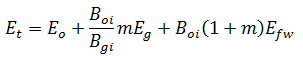
Volatile oil — Walsh formulation
Volatile oil is also called high shrinkage crude oil, or near-critical oil. It contains relatively fewer heavy molecules and more intermediates than black oils. It has a higher API (typically greater than 44), and is typically lighter in color.
A small reduction in pressure below the bubble point causes the release of a large amount of gas in the reservoir. An additional property is used to the describe volatile oil – the volatile oil ratio Rv. The volatile oil ratio describes the amount of volatilized oil in the reservoir gas phase and is typically expressed in stb/ MMscf. The volatile oil ratio is often described as "the liquid content in the gas" or the "oil vapor in the gas". An oil reservoir can be described as volatile, if the gas in the gas cap or the gas that comes out of solution contains significant quantities of volatile liquids. Volatile oils normally contain more than 500scf/ stb of dissolved gas and the liquid content of the gas phase, the volatile oil ratio, would be more than 20stb/ MMscf.
Regular material balance does not account for volatile oil. In a reservoir containing volatile oil, the Walsh formulation is used to calculate original oil-in-place. The equations which are modified from standard material balance are shown below.
| Terms | Description |
|---|---|
|
Modified withdrawal term for volatile oil. |
|
|
Modified oil expansion term for volatile oil. |
|
Modified gas expansion term for volatile oil. |