In the presence of uncertainty re: input data required for determining the best estimate of a value, probabilistic methods are used. For example, there may be uncertainty in net pay or drainage area while estimating OGIP using volumetric calculations.
Probabilistic analysis is a technique to quantify the impact of these uncertainties on output variables, and to determine a range of possible outcomes, as opposed to a single deterministic solution. The uncertainty in the output also provides a measure of the validity of the model.
The Monte Carlo simulation (using Latin hypercube sampling) is an established approach of performing a probabilistic analysis. The Monte Carlo analysis involves a large number of runs, each of which is a deterministic calculation. The inputs to these deterministic calculations are randomly drawn from probability density functions (PDFs) that describe the likely values of an input parameter. The more realistic these PDFs are, the more realistic the estimate of the output parameter, as calculated by the Monte Carlo simulation.
Probability distribution types
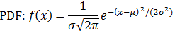
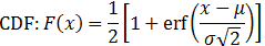
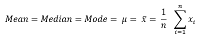
In this section, we define the different probability distribution types used as part of the probabilistic analysis. The definitions include the equations for the PDF, cumulative distribution function (CDF), mean, median, and mode for each of the probability distribution types.
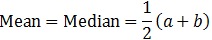
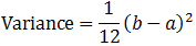
Normal distribution

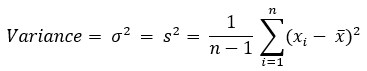
Note: The variance calculation uses the Bessel correction for bias.
Log-normal distribution

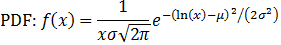
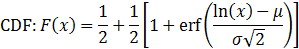
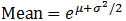
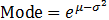
A log-normal distribution is the probability distribution of a random variable whose natural logarithm follows a normal distribution. The log of a set of data that follows a log-normal distribution follows a normal distribution. As such, it should be noted that μ is the mean of the natural log of the dataset, and σ is the standard deviation of the natural log of the dataset (that is, the mean and standard deviation of the underlying normal distribution).
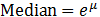
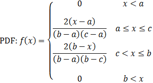
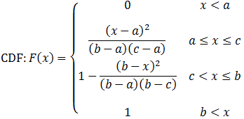
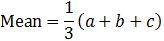
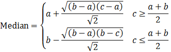
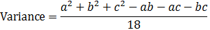
Triangular distribution
Mode = c
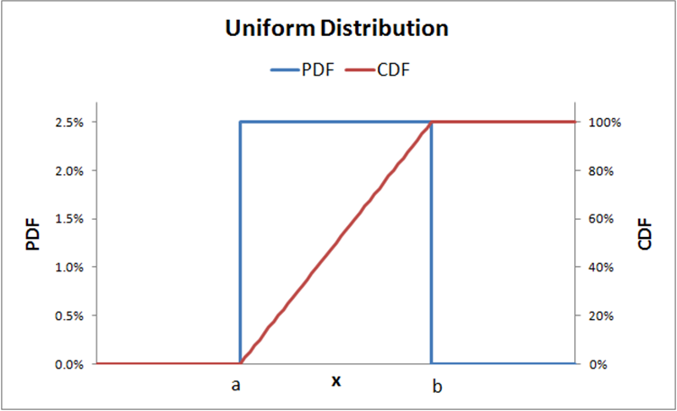
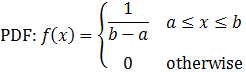
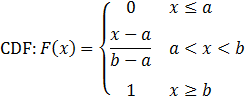
Uniform distribution

Calculation methods
Calculation methods are described below.
Monte Carlo simulation
The Monte Carlo simulation is a stochastic modeling method to simulate real-world situations where there is uncertainty in the input variables. This uncertainty cannot be directly modeled using analytical solutions. While conceptually very simple, a trivial example provides the easiest route to developing an understanding of the Monte Carlo simulation procedure.
Consider the simple estimation of prospect reserves (EUR, stbo) calculated as the product of the prospect area (A, acres), average net hydrocarbon thickness (h, feet), and recovery factor (RF, stbo/acre-ft). The algebraic expression of this simple model is:
EUR = A × h × RF
The deterministic approach would simply multiply the "best estimate" for each of these quantities to obtain a single value of EUR. The deterministic approach assumes that the most likely value of every input is encountered simultaneously, which is generally very unrealistic.
Suppose that for each of the three input variables, A, h, and RF, independent cumulative probability distributions can somehow be defined, thereby describing the uncertainty in each of these variables. The Monte Carlo method can make use of these distributions to arrive at an overall cumulative probability distribution (overall uncertainty) for EUR. This analysis approach is superior to the single-valued deterministic approach because of the valuable insight gained into the "upside," "downside," "most likely outcome," and the "mean" level of reserves that would result from drilling a large number of similar prospects.
The following describes one pass in the Monte Carlo simulation procedure:
1. Generate a random number between zero and one (representing the value of the cumulative probability) for each of the three input variables.
2. Enter the cumulative probability distribution for each input variable at their respective random number to determine the "sampled" value for each input.
3. Multiply the three independent variable sampled values to yield a sample reserve estimate.
An individual calculation or run to estimate a prospect size in this fashion is known as a "pass". By itself, the individual value of EUR generated by a pass is meaningless. However, when repeated a large number of times, a cumulative distribution for the EUR emerges.
The minimum number of passes required depends on the number of input variables that are risked. Generally, enough runs are needed to ensure that the entire domain of input variables is examined. The larger the number of input variables, the larger the minimum number of passes required.
Typically, 1000 or more passes comprise a single Monte Carlo simulation. As a qualitative rule, a smooth CDF of output variables is an indication of an appropriate number of runs.
After a Monte Carlo simulation run is finished, an analysis of the results follows. Assuming a 1,000 pass simulation run, results are processed as follows:
1. Arrange EUR results in ascending order.
2. Number the sorted EUR values from 1 to the total number of samples (for example, 1,000).
3. Calculate the cumulative probability of each value by dividing the sample number by the total number of samples (in this case, 1000).
4. Plot the resultant cumulative probability function (Cumulative Probability vs. EUR) to ascertain the smoothness of the distribution. Lacking a smooth distribution necessitates re-running the simulation with a larger number of passes.
5. Calculate the mean, variance, P10, P50, P90, and any other desired statistical parameters.
This analysis yields the statistical parameters desired for the prospect analysis. Expect the values of these parameters to vary slightly with each simulation. An unacceptably large variation warrants an increase in the number of passes.
Latin hypercube sampling
Selecting random values for model parameters can require a large number of simulation passes to generate a smooth cumulative probability distribution. Latin hypercube sampling, also known as stratified sampling, is a process applied to multiple variables to reduce the required number of passes in a Monte Carlo simulation.
First, stratified sampling is used to force randomly generated numbers to conform to the CDF represented by their statistical distribution. Normally, you could generate a random number between zero and one representing the cumulative probability a number of times, and use those numbers to read the CDF. Instead, the span of zero to one is split between the number of samples to be taken, and points within those smaller spans are randomly selected. Each of the samples is generated by:

where n is the interval index, N is the number of non-overlapping intervals, and r is a randomly generated number between zero and one (newly generated for each sample).
The effects of stratified sampling can be dramatic. The figure below compares the Cumulative Frequency Plot of 100 random samples with 100 stratified samples.
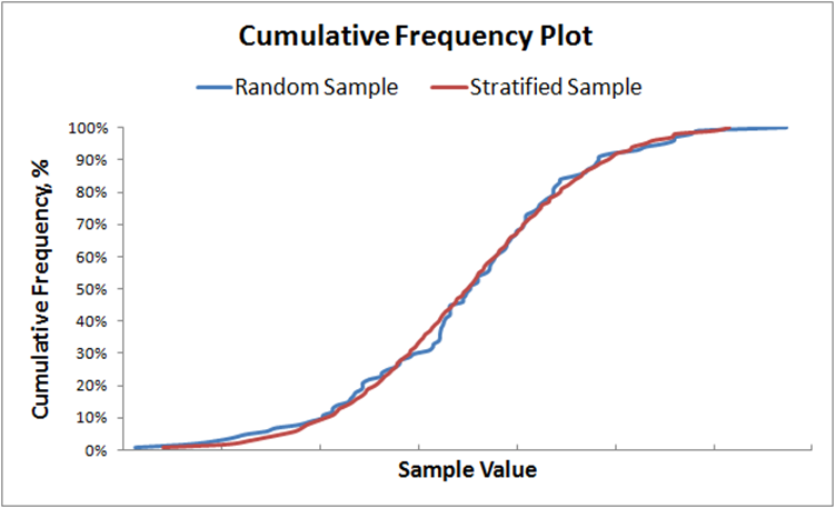
After the stratified sampling is performed on all variables, the samples are randomly grouped together to generate the parameters to be entered into the model for each simulation pass. Each value must only be used once.
Correlated sampling
This section describes methods for generating multiple sequences of correlated random variables. In other words, the values sampled in one distribution are correlated to the values sampled in another distribution, given the correlation coefficients between the two samples.
These screenshots show examples of two sequences of uncorrelated and correlated random data.
|
Two sequence of uncorrelated data: |
|
Two sequence of correlated data: |

|
|

|
Creation of correlated random variables
The rank-order correlation approach of Spearman as presented by Iman and Conover (Iman & Conover, 1982) is used to create a set of multi-variable correlated random variables.
This approach is based on using rank correlations to define dependencies among input variables. By ranking the values and using them as opposed to the actual values, the Spearman rank correlation of the input values are kept as close as possible to the target rank correlation coefficient matrix, as specified.
Because this approach is distribution-free:
- it preserves the exact form of the probability distribution functions
- it may be used with any type of distribution function
Auto-correction to user-input correlation coefficient matrix
To generate a sequence of multi-variable correlated random numbers, we need to specify the applicable matrix of correlation coefficients. This matrix is required to be positive and definite (that is, all the eigenvalues of this matrix are to be greater than zero).
If the user-specified matrix of correlation coefficients fails to qualify as a positive-definite matrix, “The Method of Eigenvalues” is used to auto-correct the matrix. Through application of slight perturbation to negative or zero eigenvalues, this method attempts to repair the correlation coefficient matrix, and make it a positive-definite one, while introducing the smallest possible changes to the matrix.
Truncated distributions
Truncated distributions are described below.
Definitions and concept
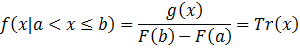
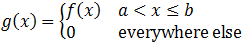
A truncated distribution is a conditional distribution that results from restricting the domain of some other distribution. In practical statistics, a truncated distribution arises from situations where the ability to record, or even know about, occurrences is limited to values which lie above or below a given threshold, or specific range.
Assuming that a random variable x has a probability density function of f(x) and a cumulative distribution function of F(x), which both have infinite support (– ∞ < x < ∞), then the probability density function after truncating the support to a < x ≤ b can be expressed as:
where:
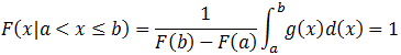
Note that Tr(x) itself is a distribution such that:
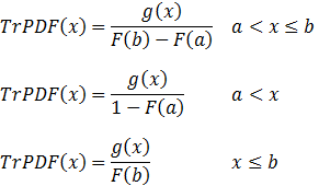
In general, the PDF of a truncated distribution function can be calculated as:
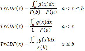
The CDF of a truncated distribution function can be calculated as:
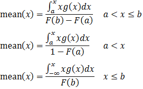
The mean of the truncated distributions are calculated as:
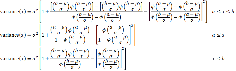
Special case: truncated normal distributions
Defining:
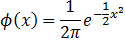
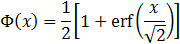
The PDF of a truncated normal distribution can be calculated as:

The mean of a truncated normal distribution can be calculated as:

The variance of a truncated normal distribution can be calculated as: