Background
The production decline analysis techniques of Arps and Fetkovich are limited in that they do not account for variations in sandface flowing pressure in the transient regime, and only account for such variations empirically during boundary-dominated flow (by means of the empirical depletion stems). In addition, changing pressure, volume, and temperature (PVT) properties with reservoir pressure are not considered for gas wells.
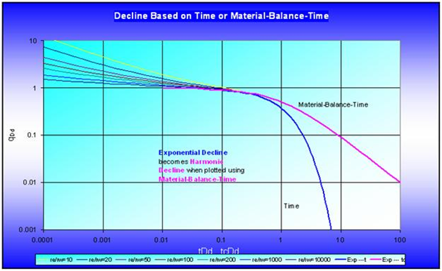
Blasingame and his colleagues have developed a production decline method that accounts for these phenomena. The method uses a form of superposition time function that only requires one depletion stem for typecurve matching - the harmonic stem. One important advantage of this method is that the typecurves used for matching are similar to those used for Fetkovich decline analysis, without the empirical depletion stems. When the typecurves are plotted using Blasingame’s superposition time function, the analytical exponential stem of the Fetkovich typecurve becomes harmonic. The significance of this may not be readily evident until considering that, if the inverse of the flowing pressure is plotted against time, pseudo-steady state depletion at a constant flow rate follows a harmonic decline trend. In effect, Blasingame’s typecurves allow depletion at a constant pressure to appear as if it were depletion at a constant flow rate. In fact, Blasingame et al. have shown that boundary-dominated flow with both declining rates and pressures appear as pseudo-steady state depletion at a constant rate, provided the rate and pressure decline monotonically.
Blasingame’s improvements on the Fetkovich style of production decline analysis are further enhanced by the introduction of two additional typecurves which are plotted concurrently with the normalized rate typecurve. These 'rate integral’ and 'rate integral derivative’ typecurves aid in obtaining a more unique match. The derivation of these will be discussed in a later section.
Blasingame in RTA
Recall that the Fetkovich typecurves are based on combining the analytical solution to transient flow of a single-phase fluid at a constant wellbore flowing pressure with the empirical Arps equations for boundary-dominated flow. Fetkovich believed the exponent ‘b’ could vary between zero and one, and that it was correlatable with fluid properties as well as recovery mechanism. For example, single-phase oil flow would result in a ‘b’ value of zero, while single-phase gas flow would exhibit ‘b’ > 0 because of changes in gas properties. Later, Fraim and Wattenbarger showed that if the changes in gas fluid properties were taken into account (i.e., with the use of pseudo-time), boundary-dominated gas flow against a constant back pressure exhibits the same behavior that an oil reservoir would; the decline would follow the exponential curve, in which ‘b’ = 0. These findings relate to flow at constant wellbore pressure. The subsequent development by Blasingame et al. was to account for changing wellbore flowing pressures by defining a superposition time function, which they called material balance time. They showed that if the material balance time were used instead of actual producing time, what was previously an exponential decline would follow the harmonic decline stem instead.
More importantly, data obtained when both the rate and the flowing pressure are varying can now be analyzed if material balance time is used. For example, if the production rate from a well is monotonically declining, and at the same time, its flowing sandface pressure is on continuous decline, a plot of pressure-drop normalized flow rate (q / ∆p) vs. Q(t) / q(t) would follow the harmonic curve (for a gas well, the changing gas properties should also be accounted for by using pseudo-time).
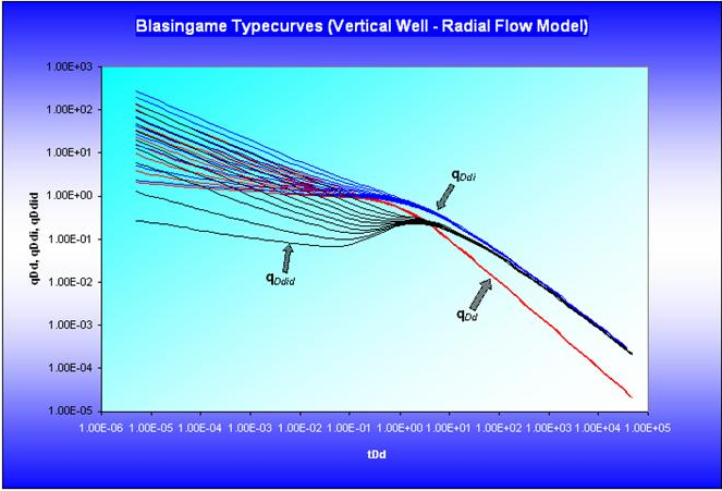
Blasingame, McCray, and Palacio developed typecurves which show the analytical transient stems along with the analytical harmonic decline (but with the rest of the empirical hyperbolic stems absent). In addition, they introduced two other functions; the rate integral function, and the rate integral derivative function, which help in smoothing the often noisy character of production data, and in obtaining a more unique match.
The Blasingame suite of typecurves are similar to the Fetkovich typecurves for constant pressure production. The only real difference is the absence of the empirical depletion stems on the Blasingame typecurves. These are not required because the usage of material balance time forces the boundary-dominated data to fall only on the analytical harmonic stem.
Models
The Blasingame suite of typecurves consists of a number of different models:
- Vertical well; radial flow model
- Vertical well; hydraulic fracture model (Infinite conductivity)
- Vertical well; hydraulic fracture model (Finite conductivity)
- Vertical well; hydraulic fracture model (Elliptical flow)
- Horizontal well model
- Waterflood model
- Well interference model (declining reservoir pressure)
All models assume a circular outer boundary, with the exception of Elliptical flow and Horizontal well typecurves, which assume an elliptical and a square outer boundary, respectively.
Methodology
In Blasingame typecurve analysis, three rate functions (normalized rate, rate integral, and rate integral derivative) can be plotted against Material Balance Time.
Normalized rate
Normalized rate is the primary plotting variable. It is very useful for production analysis where flowing pressures and rates change through time. It is defined as the rate divided by flowing pressure drop.
Oil

Gas

Rate integral
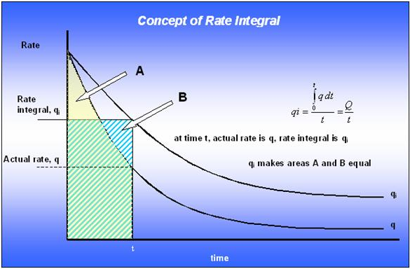
Conceptually, the rate integral may be thought of as the average rate at which the well has produced until any particular moment in time. The definition of the normalized rate integral is the cumulative average of the normalized rate when plotted against material balance time.
Surface (and even bottomhole) measured flowing rate and pressure data inherently contain a significant noise component. This noise often masks or distorts the sought after "reservoir signal". As a result, it is advantageous to have a way to remove this noise from the production data response.
Blasingame has identified a powerful method for removing noise from a production response, by using integration. The rate integral (the inverse of this is the pressure integral) is referred to as an auxiliary function, and is derived by integrating the normalized production rate response through time. Any discontinuities in the raw data are effectively removed through the integration process, yielding a smooth decline curve. The resulting curve resembles the original production decline response, but is much smoother. It can be used to perform a secondary typecurve match (simultaneously with the raw data). Furthermore, it may be used as base data for a well-test style semi-log derivative plot.
Conceptually, the rate integral function can be thought of as a cumulative average of the flow rate with time. The purpose of plotting a rate integral function is to smooth noisy rate data. This concept is most easily understood graphically:
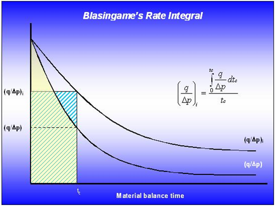
In terms of Blasingame typecurve analysis, the definition of the rate integral must account for two additional complications:
- Normalization of flow rate using pressure (for oil) or pseudo-pressure (for gas)
- Usage of material balance time (for oil) or material balance pseudo-time (for gas), instead of time
Oil

Gas

Rate integral derivative
The rate integral derivative is defined as the semi logarithmic derivative of the rate integral function, with respect to material balance time.
Oil

Gas

Calculation of parameters
The actual normalized rate, rate integral, and rate integral derivative are plotted vs. material balance time data on a log-log scale of the same size as the typecurves. This plot is called the data plot. Any convenient units can be used for normalized rate or time because a change in units simply causes a uniform shift of the raw data on a logarithmic scale. It is recommended that daily operated-rates be plotted, and not the monthly rates, especially when transient data is analyzed. Any one of the curves can be used individually but often using more than one curve helps in achieving a more unique match of the data with the typecurves.
Move the data plot over the typecurve plot, while the axes of the two plots are kept parallel, until a good match is obtained. The rate, rate integral, and rate integral derivative data should all fit the same corresponding typecurve. Try several different transient typecurves to obtain the best fit of all the data. Select the typecurve that best fits the data, and note and its re / rwa value.
Typecurve analysis is done by selecting a match point and reading its coordinates off the data plot (q / ΔP and tc for oil, q / Δpp and tca for gas) match; and off the typecurve plot (qDd and tDd) match. Note the stem value re / rwa of the matching curve.
Given a curve match, the following reservoir parameters can be obtained if reservoir thickness, total compressibility, and wellbore radius are known:
- Permeability
- Skin
- Fracture half length
- Dimensionless fracture conductivity
- Area
- Original oil- or gas-in-place
To create a forecast, the selected typecurve is traced on to the data plot, and extrapolated beyond the last data points. The future rate is read from the data plot, off the traced typecurve.
| Note: | The above calculation parameters reflect a vertical well with a radial flow model. Selection of other typecurve models for matching requires some adjustments. For information on other model calculation parameters, see transient typecurve matching equations. |
Boundary-dominated flow
Harmonic stem of decline curves
Recall from the derivation of Material Balance Time:

Taking the reciprocal and rearranging provides the same form as the harmonic branch of Arps typecurve:

To further show the similarity to the harmonic equation, the equation above can be written as follows:

where:


The rearranged material balance time equation is significant; if the pressure-drop normalized flow rate is plotted vs. material balance time, the data will follow the harmonic branch of the Fetkovich or Arps typecurve (regardless of whether production is constant or variable flow rate, or constant or variable sandface pressure).
The relations that are used to compute oil-in-place and reservoir properties are given by Equations A14-A16 of Palacio and Blasingame (1993).


Data preparation
In Blasingame typecurve analysis, boundary-dominated flow is represented by a single harmonic stem, into which all the transient stems converge.
To calculate original gas-in-place and original oil-in-place, the plotted data are matched against the harmonic stem, which is defined mathematically as follows:

Oil
where:

and:

The pseudo-steady-state equation for oil in decline form is as follows:

Through comparison of (1) and (3), it is clear that a graph of normalized rate vs. material balance time will follow the trend of the dimensionless harmonic stem.
From equations (1), (2), and (3) we get the following:

where:


Solving for N, we get:

Gas
The development for gas is similar to that of oil. However, pseudo-pressure and pseudo-time must be used in place of pressure and time.
The definitions of the dimensionless variables are as follows:

and:

The pseudo-steady-state equation for gas is as follows:

Combining equations (1), (6) and (7):

where:

and:

Solving for G, we get:

Transient typecurve matching equations
The evaluation of transient parameters is accomplished using the transient stems of the dimensionless typecurve model. Unlike the boundary-dominated flow case, the definition of the characteristic dimensionless variables changes according to the chosen transient model. Presented in this section are the typecurve matching equations for five different transient models:
- Radial (Vertical Well)
- Infinite Conductivity Fracture
- Finite Conductivity Fracture
- Horizontal Well
- Elliptical Flow Typecurves
The typecurves are plotted using the dimensionless decline rate qDd and dimensionless decline time tDd, which are defined as follows:

where:


where:


The dimensionless pseudo-steady state constant bDpss is defined differently for each model.
Radial
The radial model simulates a vertical well in the center of a cylindrical reservoir.
The characteristic dimensionless parameter reD = re / rwa represents the ratio of the external reservoir radius to the apparent wellbore radius.
The dimensionless pseudo-steady state constant bDpss is defined as follows for the radial model:

Oil
Permeability is obtained by rearranging the definition of dimensionless decline rate:


Solve for apparent wellbore radius from the definition of dimensionless decline time:


Skin is calculated as follows:

Gas
Permeability is obtained by rearranging the definition of dimensionless decline rate:


Solve for apparent wellbore radius from the definition of dimensionless decline time:


Skin is calculated as follows:

Infinite conductivity fracture
The fractured model simulates an infinite conductivity hydraulic fracture (vertical) in the center of a cylindrical reservoir.
The characteristic dimensionless parameter reD = re / xf represents the ratio of external reservoir radius to fracture half-length.
The dimensionless pseudo-steady state constant is defined as follows for the infinite conductivity fracture model:

Oil
Permeability is obtained by rearranging the definition of dimensionless decline rate:


Solve for effective radius from the product of dimensionless decline rate and dimensionless decline time:

Solve for fracture half-length from the definition of dimensionless effective radius:

Gas
Permeability is obtained by rearranging the definition of dimensionless decline rate:


Solve for effective radius from the product of dimensionless decline rate and dimensionless decline time:

Solve for fracture half-length from the definition of dimensionless effective radius:

Finite conductivity fracture
A fracture with finite conductivity is defined as a planar crack penetrated by a well or propagated from a well by hydraulic fracturing having a non-zero pressure drop in the fracture during production. A fracture with finite conductivity is characterized by dimensionless fracture conductivity which is defined as:

For FCD > 50, the fracture is assumed to have infinite conductivity. The finite conductivity fracture model in RTA simulates a vertical fracture in the center of a cylindrical reservoir. The characteristic parameter reD = re / xf represents the ratio of external reservoir radius to fracture half length.
The dimensionless pseudo-steady state constant bDpss is defined as follows for the finite conductivity fracture model:

where:
u = ln(FCD)
a1 = 0.936268
a2 = -1.00489
a3 = 0.319733
a4 = -0.0423532
a5 = 0.00221799
b1 = -0.385539
b2 = -0.0698865
b3 = -0.0484653
b4 = -0.00813558
Oil
Permeability is obtained by rearranging the definition of dimensionless decline rate:


Solve for effective radius from the product of dimensionless decline rate and dimensionless decline time:

Solve for fracture half-length from the definition of dimensionless effective radius:

Additional parameters are then calculated using the following equations:


Radial flow skin factor:

where:
 .
.
Gas
Permeability is obtained by rearranging the definition of dimensionless decline rate:


Solve for effective radius from the product of dimensionless decline rate and dimensionless decline time:

Solve for fracture half-length from the definition of dimensionless effective radius:

Additional parameters are then calculated using the following equations:


Radial flow skin factor:

where:
u = ln(FCD)

Horizontal well
The horizontal well's typecurve-matching procedure is based on a square-shaped reservoir with uniform thickness (h), and the well is assumed to penetrate the center of the pay zone. Note that the horizontal well typecurve does not include any options for including hydraulic fractures.
The procedure for matching horizontal wells is similar to that of vertical wells. However, for horizontal wells, there is more than one choice of model. Each model presents a suite of typecurves representing a different penetration ratio (L / 2xe) and dimensionless wellbore radius (rwD). The definition of the penetration ratio is illustrated in the following diagram:

The characteristic dimensionless parameter for each suite of horizontal typecurves is defined as follows:

where β is the square root of the anisotropic ratio:

The dimensionless pseudo-steady state constant bDpss is defined as follows for the horizontal well model:

where:
γ = Euler's constant = 0.57721
Oil
Dimensionless decline rate is defined differently for horizontal oil wells, than for the radial or fractured cases:

Horizontal permeability (kh) is obtained by rearranging the above definition of dimensionless decline rate:

Vertical permeability (kv) is calculated using the anisotropic ratio:

Gas
Dimensionless decline rate is defined differently for horizontal gas wells, than for the radial or fractured cases:

Now, permeability is obtained by rearranging the above definition of dimensionless decline rate:

Vertical permeability is calculated exactly the same as for the oil case, using the anisotropic ratio.
Elliptical flow typecurves
Elliptical flow is considered to be the governing flow regime for low permeability gas reservoirs when the reservoir has some sort of an elliptical outer or inner boundary. Cases such as production from an elliptical wellbore, an elliptical fracture, or a circular wellbore in an anisotropic reservoir system can be considered to be examples of an elliptical inner boundary. An elliptic reservoir surrounded by an elliptic aquifer is the example of an elliptical outer boundary.
The elliptical flow typecurves in RTA are generated for a hydraulically fractured well in the center of a reservoir with a closed elliptical boundary.
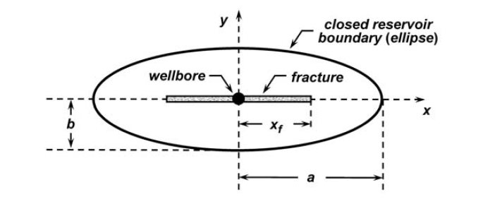
Schematic of the elliptical reservoir model (Amini et al. 2007).
The following assumptions are made in order to develop these typecurves (Amini et al. 2007):
- The reservoir is assumed to be a single-layer system that is isotropic, horizontal, and uniform thickness with constant reservoir characteristics.
- The fracture is assumed to have elliptical shape. It is also assumed that the fracture is very narrow compared to length of the fracture.
- The elliptical outer boundary is assumed to have a focal length equal to fracture half length.
In the case of infinite conductivity fracture, we do not need to consider the flow in the fracture because of constant pressure along the fracture. However, when we are dealing with a finite conductivity fracture, the flow through fracture should be considered, as the pressure drop within the fracture becomes significant compared to the total pressure drop of the fracture and reservoir. In this case, we should solve the diffusivity equations for reservoir and fracture. However, these equations cannot be solved separately and they are coupled together. In the following sections the diffusivity equation, as well as initial and boundary conditions for reservoir and fracture domains are presented.
Calculation of parameters
Oil wells
Using the definition of dimensionless rate for oil wells:

Permeability is calculated as follows:

From the definition of area-based dimensionless time (tDA) for oil wells:

Area is calculated as follows:

Substituting the equation for permeability into the above leads to:

Additional parameters are then calculated using the following equations:


Gas wells
Using the definition of dimensionless rate for gas wells:

Permeability is calculated as follows:

From the definition of area-based dimensionless time for gas wells:

Area is calculated as follows:

Substituting the equation for permeability into the above leads to:

Additional parameters are then calculated using the following equations:


