The transient typecurve analysis method provides an alternative perspective that is ideal for analysis of very short (early) production periods, and/or analysis of very low permeability reservoirs.
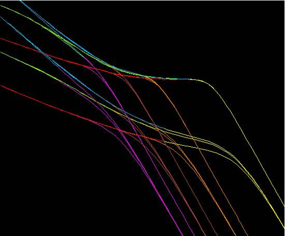
In the Blasingame, Agarwal-Gardner and Normalized Pressure Integral methods, the typecurves are scaled such that there is convergence onto a single boundary-dominated stem (unit slope). This is achieved through the use of a dimensionless time that is based on area (tDA or tDd). One consequence of this type of scaling is that there are numerous transient stems. If a dimensionless time based on well radius (tD) is chosen instead, there will be a single transient stem with a series of boundary-dominated curves. When viewing a single typecurve (e.g., reD = 28) there is no difference between these two scaling formats (see figure below). However, when viewing all the typecurves together, the transient presentation provides a more convenient base for analysis of transient data. This follows from the fact that selection of an appropriate transient stem is not required.

Consider a transient production data set (either very low permeability, or limited production life). A comparison of the typecurve match using Agarwal-Gardner Rate-Time analysis with that of the Transient format is shown below.

It is clear from this example that the transient presentation of the typecurves provides a more unique typecurve match. For the same reason that transient data works better with the transient format (qD vs. tD), it should be noted that boundary-dominated flow analysis is not advised using this method.
The accepted time-superposition function for Rate Transient Analysis is material balance time. Since material balance time is rigorous for boundary-dominated flow, it is a natural standard for evaluating variable rate production data. However, when dealing with transient data, it is clearly not the best option. The standard time-superposition for transient flow (pressure transient analysis) is radial-superposition time. When using the transient typecurves in RTA, both the radial and linear superposition time options are available.
Inverse pressure integral derivative
This derivative can make typecurve matching easier by exaggerating features in the data. In most cases, the inverse pressure derivative was found to be too sensitive to be useful. The inverse pressure integral derivative is less sensitive and so can be interpreted more handily, while still providing detail about the character of the data.
We start with dimensionless pressure:

Next we define the dimensionless pressure integral:

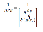
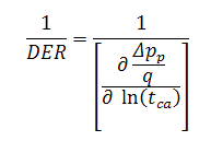
This is used to define the inverse pressure integral derivative:

This can also be written as:

Data preparation
The horizontal axis is material balance time (pseudo-time for gas).
On the vertical axis, two variables are plotted:
- Normalized Rate vs. Material Balance Time
- Inverse of Semi-log Derivative vs. Material Balance Time
Normalized rate
Oil wells


Gas Wells


| Note: | In the modified (RTA) plot, the 1 / DERi (inverse pressure integral derivative) is also included. |
Analysis
The normalized rate and inverse semi-log derivative data are plotted against material balance time on a log-log scale of the same size as the typecurves. This plot is called the "data plot". Any convenient units can be used for normalized rate or time because a change in units simply causes a uniform shift of the raw data on a logarithmic scale. It is recommended that daily operated-rates be plotted, and not the monthly rates; especially when transient data are analyzed.
The data plot is moved over the typecurve plot, while the axes of the two plots are kept parallel, until a good match is obtained. Several different typecurves should be tried to obtain the best fit of all the data. The typecurve that best fits the data is selected and its "re / rwa" (re / xf for fractured case) value is noted.
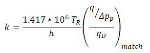
Typecurve analysis is done by selecting a match point, and reading its coordinates off the data plot (q / Δp and tc) match, and off the typecurve plot (qD and tD) match. At the same time the stem value "re / rwa" (re / xf for fracture typecurves) of the matching curve is noted.
To create a forecast, the selected typecurve is traced on to the data plot, and extrapolated. The future rate is read from the data plot, off the traced typecurve.
Calculation of parameters: radial typecurves
Oil wells
Permeability is obtained by rearranging the definition of dimensionless rate:


Solve for apparent wellbore radius from the definitions of dimensionless time and permeability:

Skin factor is calculated as follows:

Volume and area parameters are calculated as follows:


Gas wells
Permeability is obtained by rearranging the definition of dimensionless rate:


Solve for apparent wellbore radius from the definitions of dimensionless time and permeability:

Skin factor is calculated as follows:

Volume and area parameters are calculated as follows:


Calculation of parameters: finite conductivity fracture typecurves
The finite conductivity fracture typecurves are based on a square-shaped reservoir with a hydraulic fracture in the center. They are plotted using dimensionless time format, and are therefore categorized as transient format curves. The transient stems represent three different dimensionless fracture conductivity (FCD) values (0.5, 5, and 500). The boundary dominated stems diverge at each of four (1, 2, 5, 25) dimensionless reservoir length (xeD) values.

Definitions
Dimensionless fracture conductivity:

Dimensionless reservoir length / width:

Where 2Xe = primary reservoir dimension
Oil wells
Permeability is obtained by rearranging the definition of dimensionless rate:


Solve for fracture half-length from the definitions of dimensionless time and permeability:

Volume and area parameters are calculated as follows:


Gas wells
Permeability is obtained by rearranging the definition of dimensionless rate:


Solve for fracture half-length from the definitions of dimensionless time and permeability:

Volume and area parameters are calculated as follows:

