Unconventional reservoir analysis

The unconventional reservoir module (URM) analysis is used to identify linear and/or boundary-dominated flow regimes within your data. Additionally, this analysis generates production forecasts for shale or tight oil / gas wells. This analysis requires sandface flowing pressures, production rates, and reservoir / fluid parameters. If the required pressures, rates, and properties are not filled in, the parameters pane of the analysis is disabled. For more information on the calculations, see unconventional reservoir theory.

Note: This analysis works with your Harmony Reservoir™ license.

This analysis has the following solution options:

Constant Pressure — the constant pressure solution for a basic linear flow model. An analysis line is fit to the data on a Reciprocal Rate vs Square Root Time plot. The slope and y-intercept of the analysis line are used to determine the linear flow parameters, along with apparent skin or apparent fracture conductivity, respectively.
Variable Pressure — the constant rate solution for a basic linear flow model. An analysis line is fit to the data on a Normalized Pressure vs Square Root Time plot. This accounts for changing flowing pressures when interpreting the slope of the square-root time plot. The slope and y-intercept of the analysis line are used to determine the linear flow parameters, along with apparent skin or apparent fracture conductivity, respectively.

Superposition Time — the superposition of the constant rate solution for a basic linear flow model applied over time to account for variations of rate over time. An analysis line is fit to the data on a Normalized Pressure vs Linear Superposition Time plot, or Material Balance Time plot, depending on the time option selected in the parameters pane. The slope and y-intercept of the analysis line are used to determine the linear flow parameters, along with apparent skin or apparent fracture conductivity, respectively.
Deterministic — creates an analysis based on known parameters.
Most Likely — creates an analysis based on a range of values, and produces "most likely" values that can be used to estimate model parameters.

Note: The production forecast for the variable pressure and superposition worksheets is estimated using constant sandface pressure (p_wff).

Tip: For a multiphase oil URM analysis, pseudo-pressure is used instead of pressure. This may impact your data-point selection, if you manually best fit your data points with Harmony Enterprise 2017.3 or earlier, and selected the Changing Properties (Pseudo-Pressure) checkbox. It is now called the Multiphase (Pseudo-Pressure) checkbox.

Unconventional Reservoir pane

In the Unconventional Reservoir pane, enter the required parameters and select your options.

Parameters

Parameters include the inputs you specify, or the default Harmony Enterprise values and calculated values from the plot interpretations.

Additional gas options for adsorption and geomechanical models can be used by clicking their checkboxes. These model options require that the Langmuir isotherm and permeability and/or compressibility ratio correlations be entered in the Properties editor.

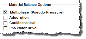
Multiphase (Pseudo-Pressure) — accounts for the variation of oil properties with pressure. Calculations use the Oil properties that are set in the Properties editor.
Adsorption — includes the effect of adsorbed gas.
GeoMechanical — accounts for the variation in rock properties (permeability and formation compressibility) with pressure. Calculations use the rock properties that are set in the Geomechanical section of the Properties editor. Note that for the Oil URM analysis, this option is only available when the Multiphase (Pseudo-Pressure) option is selected.
PSS Water Drive — accounts for pseudo-steady state (PSS) water drive (additional water drive analysis parameters are displayed).

The flowing pressure inputs in the Forecast parameters section are used with the slope of the Square Root Time plot to determine xf√k. You can enter the drainage area, or area of SRV, but by default, these values come from the OOIP / OGIP on the flowing material balance (FMB) plot. Changes to the location of the end of linear flow line (t_elf ) on the Square Root Time plot updates the OOIP / OGIP. The decline exponent, b, and the final gas rate are used to calculate the hyperbolic decline forecast. The start date is the end of production data for the well. The ∆t is set based on the forecast duration to reach the final rate, and corresponds to the end date. Either q_f or ∆t can be entered, and the other value is calculated.

Forecast Parameters

The second half of the parameters pane displays calculated values from the interpretations:

The x_{f total} √k_SRV is determined from the slope of the analysis line on the Square Root Time plot. Here k is effective permeability to the primary fluid (that is, oil for Oil URM, gas for Gas URM).
The x_{f total} √k_SRV(Abs) is calculated based on x_{f total} √k_SRV, using the relation between effective and absolute permeability: k_SRV = k_SRV(Abs) k_rx (S_xi) where k_rx (S_xi) is a relative permeability of the primary fluid at initial saturation.
The time to reach the end of linear flow (t_elf) is determined from the position of the t_elf line on the Square Root Time plot.
The OOIP / OGIP displayed is related to the area used.
The EUR and RR come from the boundary-dominated flow Forecast plot.

Calculations

Additional parameters depend on the Model Type you select:

Vertical - Single Frac — if you type a value for k_SRV, x_f is calculated based on it.
Hz - Multi Frac - Effective k — the stimulated region is treated as a region of higher effective permeability, and the observed linear flow is interpreted as flow towards the wellbore. Therefore, the linear flow parameter obtained from the slope of the analysis line is interpreted as: A_c √k_SRV = 2 L_e h √k_e. If you type a value for L_e, k_e is calculated.
Hz - Multi Frac - SRV — this model considers bi-wing fractures extending from the horizontal well, and the area of the stimulated region is based on the FMB interpretation. If you type a value for L_e and n_f, x_f is calculated based on the area (A_SRV = 2 L_e x_f). Then, k_SRV is calculated based on x_f (x_{f total} √k_SRV = n_f x_f √k_SRV).

Note: None of the inputs in the Calculations section are required, but the inputs provide additional information about the model used for forecasting.

Primary toolbar

The primary toolbar is located in the Unconventional Reservoir pane and has these icons:

Apply Defaults — copies parameters These parameters can be copied from one unconventional analysis to another: -fracture height min & max -model type (fracture mode) -changing properties options: geomechanical, changing oil saturation, use pseudo-time -material balance options: adsorption, geomechanical -superposition time options: (superposition time type) -forecast parameters: b, qf -typecurve options: raw derivative status, derivative status from the Properties editor or other IHS Reservoir worksheets.
Change Top Left View — select a plot to be displayed in the top left of your dashboard.
Change Top Right View — select a plot to be displayed in the top right of your dashboard.
Change Bottom Left View — select a plot to be displayed in the lower left of your dashboard.
Change Bottom Right View — select a plot to be displayed in the lower right of your dashboard.
Float a New View — select a plot to be displayed in a new floating window.
Save or Erase Default Dashboard — select either save (to save your current dashboard configuration as the default setting), or reset (to reset the dashboard to its original settings).
/ Show / Hide Disabled Points — toggle between showing / hiding disabled points on your plot.

For a description of common toolbar icons, see toolbars.

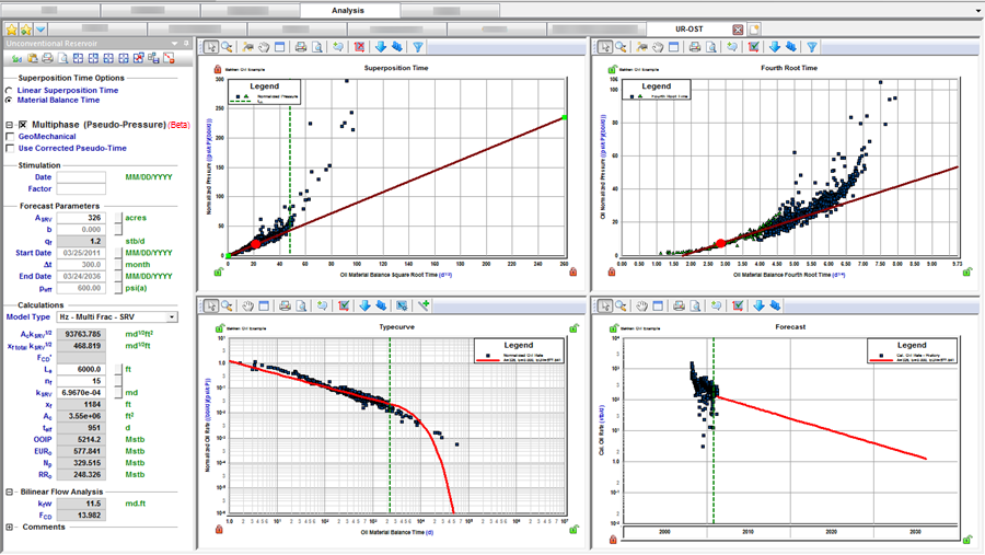
Plot dashboard

The plot dashboard displays your four favorite plots.

Note: For the FMB plot on the dashboard, the OGIP is anchored to the x-axis as a pivot point, and you can move the y-axis intercept by clicking-and dragging the green square. The anchored point on the x-axis is dictated by the t_elf line on the Square Root / Superposition Time plot.

Plot toolbar

The icons displayed in the plot toolbar vary depending on the type of plot that you have displayed. The important icons are described below.

Single Annotation — adds an annotation arrow to the data point you click.
Linked Annotations — synchronizes your annotation arrows across unconventional reservoir plots. For example, if you move your annotation on one plot using the keyboard arrow keys, the arrow is synchronized on the other plots. The values vary as you move from the displayed date for one date / time row in the Production editor to the other.
Data Filter — opens the Data Filter dialog box where you can apply a data filter. For more information, see saturated filter.
Boundary Dominated Curve — applies a boundary-dominated curve to your plot.
Typecurve Options — opens the Typecurve Options dialog box where you can toggle the Raw Data Derivative and Beta Derivative options, as well as select your derivative type (Standard, Bourdet, or Difference) and derivative cycles. For bilinear flow, the beta-derivative is 0.25; for linear flow, it is 0.5; for boundary-dominated flow, it is 1.0.

For a description of common plot icons, see plot toolbars.