Numerical URM theory

The numerical unconventional reservoir model (URM) analysis was developed based on URTeC-2020-2967-MS and accounts for multiphase behavior, including total compressibility change when pressure drops below saturation pressure. Similar to the traditional URM analysis, numerical URM is used to determine the following: the linear flow parameter (LFP or Ac √k) and the size of SRV (A_SRV or OFIP_SRV.

Summary of methodology

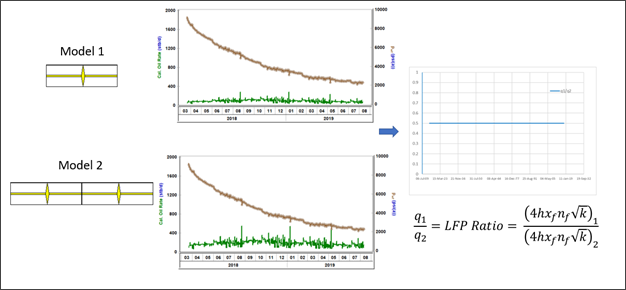
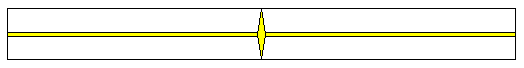
Consider two similar models for a horizontal multi-fractured well. Both models have:

• SRV geometry (exhibit linear flow followed by boundary dominated flow)
• same initial pressure
• same PVT properties
• same relative permeability curves
• same porosity and initial saturations
• pressure control calculation (using same historical pressures)

However, these two models may have different LFP (Linear Flow Parameter = 4hx_f n_f √k).

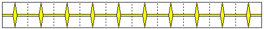
This can be visualized as two models where just the number of fracture stages n_f is different (but the same would apply if h, x_f, or k are different).

In this case, rates produced by these two models are proportional to their LFP ratio:

Now we use this concept to analyze actual well data. We build any model to use as model 1 (as long as it has SRV geometry and stays in linear flow); this model will have the same PVT properties, relative permeabilities, initial pressure, and saturations as the well being analyzed. We call this model the Base Model. LFP for the Base Model is known. The Base Model is calculated with pressure control to obtain q_BaseModel rates.

Instead of model 2, we use the actual historical production data of the well:

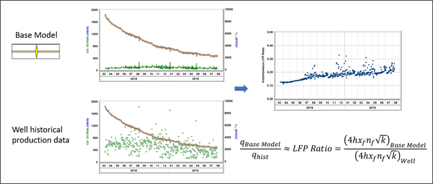
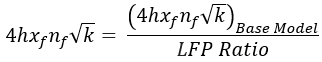
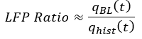
The LFP ratio can then be estimated from the dataset (plotted against time), and then LFP of the well can be calculated as:

The LFP of the well is the main output from Numerical URM analysis.

Additional outputs, options, and calculations are described in detail in the subsequent sections.

Assumptions

The analysis are done on a production dataset (rates and flowing pressures) for a horizontal multifrac well. It is assumed that the dataset being analyzed can be modeled closely using a numerical model. This model is referred to as the history-matched model (HM model). It is assumed that the following is true about this model:

• Model geometry is supposed to be an SRV geometry; therefore a linear flow regime is expected for the well followed by boundary-dominated flow.
• 
• Initial reservoir pressure, PVT properties, and relative permeabilities are assumed to be known (should be entered in the Properties editor).
• Geological parameters such as porosity, net pay, saturations, rock compressibility, and pressure-dependent permeability are assumed to be known (should be entered in the Properties editor.
• Other model parameters such as LFP (Ac √k), k_SRV, t_elf, x_f, and OFIP_SRV are unknown and can be estimated using the numerical URM analysis.

Essentially, the numerical URM analysis assumes that well behavior can be closely described by the HM model, and gives parameters of this HM model as output.

Estimating the LFP

To estimate the linear flow parameter (LFP) of the HM model:

1. In the background, a base linear model (BL model) is created. It is a numerical model that has the same PVT properties, relative permeabilities, and geological properties as the HM model. The geometry of this base model should represent an SRV model with:

• A known p_i, PVT, and geological properties
• Only one fracture
• High fracture conductivity
• No outside flow (2x_f = reservoir width)
• Single permeability (k_SRV = k_matrix)
• Large lateral length (L_e) so that the base model remains in linear transient flow for the entire simulation
• 

2. Run the BL model at pressure control using the actual drawdown of the well being analyzed.

Equation 1: Pressure drawdown for each timestep is proportional to rate

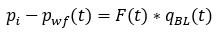
where q_BL (t) are synthesized rates using the BL model (run at pressure control).

During the first transient linear flow, you can think of the HM model as of multiple stages of the BL model. Therefore, if the HM model is also simulated at pressure control, the HM model produces rates that are proportionally higher than the BL model's rates. (The proportion of the rates is defined by the LFP ratio of both models.)

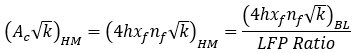
Equation 2

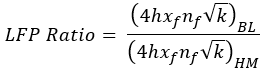
where (4hx_f n_f √k)_BL is the LFP of the BL model and (4hx_f n_f √k)_HM is the LFP of the HM model.

The LFP ratio describes the performance ratio of the BL and HM models during transient linear flow.

Equation 3: During transient linear flow

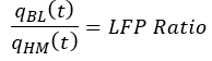
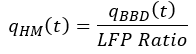
where q_HM (t) are synthesized rates using the HM model (run at pressure control).

During the first transient linear flow, pressure drawdown for the HM model at each timestep can be obtained by combining equations 1 and 3.

Equation 4

Assuming the HM model describes the production history closely enough,

Equation 5

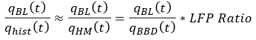
during transient linear flow, combining equations 3 and 5:

Equation 6

where q_hist (t) are historical rates observed by the well.

Equation 6 is used to build the Multiphase Diagnostic plot where is plotted against time.

These points are supposed to approximately follow a flat trend during the first transient linear flow regime. The position of the flat line (Y-intercept) gives the value of the LFP ratio.

Since all parameters of the BL model are known, (4hx_f n_f √k)_BL is also known, therefore the LFP of the HM model can be calculated using equations 2.

Equation 7: Main outcome of the numerical URM analysis

Additionally, the same plot can be used to estimate the time to the end of linear flow (t_elf). The BL model stays in a transient linear flow regime throughout the entire production history, while the actual well may transition to boundary-dominated flow at some point.

At this time, starts to increase. Therefore, the time when points on the Multiphase Diagnostic plot start curving upward from the flat trend indicates the end of the first transient linear flow.

Parameter breakdown

Similar to the traditional URM, the numerical URM analysis does not immediately give values for individual completion parameters. Instead, the combined parameter of A_c √k = 4hx_f n_f √k is estimated. Individual parameters can be calculated assuming that other parameters are known. LFP can be broken down into completion parameters using one of the following two ways:

• k is calculated by entering n_f and x_f , using h from the Properties editor, and A_c √k
• x_f is calculated by entering n_f and k, using h from the Properties editor and A_c √k

Estimating OFIP

While the BL model stays in transient linear flow throughout the entire production history, the actual well may reach boundary-dominated flow. After this happens, points on the top-left plot start curving upwards. The HM model is assumed to match both the transient linear and the boundary-dominated portion of data. To analyze the boundary-dominated portion of data, additional adjusted base model data is built and run in the background. The adjusted base model is the same as the BL model except it uses a smaller L_e such that the model reaches boundary-dominated flow during simulation time. The adjusted model is referred to as the base boundary-dominated model (BBD model).

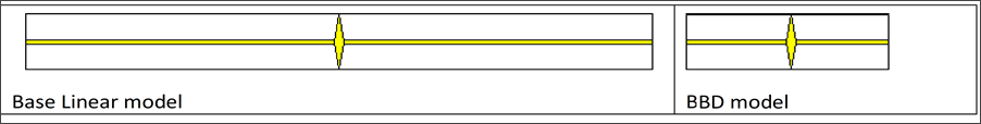
The size of the BBD model should be such that transition from the transient linear flow to the boundary-dominated flow happens at the same time as it happens for the HM model. This is achieved by trial and error on OFIP_SRV and ultimately L_e of the BBD model.

Equation 8

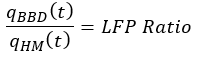
Note that this relationship is true not just during the transient linear flow, but throughout the entire production history.

Assuming that the HM model describes the production history closely enough, q_HM (t) ≈ q_hist (t), therefore:

Equation 9

To add results from the HM model on the Multiphase Diagnostic plot, the BBD model is run at pressure control and q_BBD (t) is calculated for each timestep; then is plotted (red curve).

History matching the boundary-dominated portion of the data is done by adjusting the BBD model until:

• Both the BBD model and historical data have the same t_elf (red line and data points start curving upwards at the same time).
• The HM model matches the boundary-dominated portion of the data (there is a match between the red line and the points on the top-left plot).

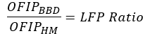
After the match is achieved, (OFIP)_BBD can be used to calculate (OFIP)_HM using this relationship:

Equation 10

Note:   History matching the boundary-dominated portion of the data is done by trial and error. For each OFIP_SRV, Harmony Enterprise first calculates OFIP_BBD using equation 10, and then calculates L_e for the BBD model. The q_BBD (t) is calculated by synthesizing the BBD model and the HM model results are updated using equation 9.

After the boundary-dominated portion of the data is matched, if the match seems reasonably unique, the OFIP_SRV can be used to calculate individual completion parameters (x_f and k_SRV). Harmony Enterprise calculates x_f based on OFIP_SRV and L_e. Then, permeability is calculated based on this x_f and LFP.

History match plot

After both the liner and boundary-dominated portions of data are matched, equation 8 can be rearranged to solve for q_HM (t):

Equation 11

q_HM (t) and q_hist (t) are plotted together against time in the lower-left plot.

Accounting for additional pressure drop (low F_CD)

Sometimes wells exhibit additional pressure drop. This additional pressure drop may be due to damage around the fracture, low fracture conductivity (F_CD), cleanup, or other reasons. In the Multiphase Diagnostic plot, this pressure drop indicates a decreasing portion of the data at the start of production.

If this additional pressure drop behaves as a pressure drop due to skin (that is, it is proportional to the primary rate), it can be accounted for.

If we define a damage factor for the well as ∆P_s, additional pressure drop due to skin at each time can be expressed as ∆P_s *q_hist (t). Therefore, equation 4 can be modified as:

Equation 4a

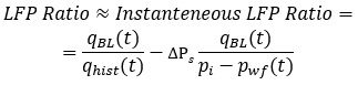
Combining equations 1 and 4a and using q_HM (t ) ≈ q_hist (t), the LFP ratio can be expressed as:

Equation 6a

This can be rearranged as:

Equation 12

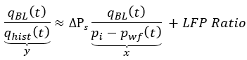
Equation 12 is used to build the Effect of Skin plot: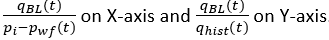

The portion of the data corresponding to early flow follows a straight line with the slope of ∆P_s and the intercept of the LFP ratio.

The Multiphase Diagnostic plot should also be modified following equation 6a by plotting 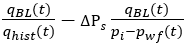against time.

During the first linear flow, these points are supposed to approximately follow a flat line. The position of the line gives the value of the LFP ratio.

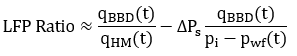
Equation 6a can be modified for boundary-dominated flow assuming q_HM (t ) ≈ q_hist (t):

Equation 13

Equation 13 can be rearranged and solved for q_HM (t):

Equation 11a

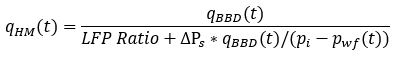
Equation 11a is used to calculate the rate for the HM model (History plot).

Note that the above derivation is all done under the assumption that the additional pressure drop is proportional to the primary rate. In reality this may not always be the case, so you should use this correction with caution. We recommend using this correction only if you see:

• a decreasing slope at the start of production on the Multiphase Diagnostic plot, and
• a clear increasing linear trend on the Effect of Skin plot, and
• a decreasing slope at the start becomes more flat after the correction is applied