Pressure loss calculations

In order to have flow in a pipe system, a pressure difference is needed, as fluids flow from a high pressure point to a low pressure point. You can identify three components that define this pressure difference:

1. Hydrostatic pressure loss

2. Frictional pressure loss

3. Kinetic pressure loss

For most applications, kinetic losses are minimal and can be ignored. Thus, the equation that describes the overall pressure losses can be expressed as the sum of two terms:

ΔPT = ΔPHH + ΔPf

Note:   The phrases "pressure loss," "pressure drop," and "pressure difference" can be used interchangeably.

In upward (or “uphill” in the context of pipelines) flow, fluids must overcome the back-pressure exerted by the effective column of fluid acting against the direction of flow. Fluids must also overcome friction losses due to the interaction of the fluid with the pipe wall.

In downward (or “downhill” in the context of pipelines) flow, friction effects act against the direction of flow, but in this case, the effective hydrostatic column helps the fluid to overcome such friction losses.

Hydrostatic pressure losses are a function of the density of the fluid in the pipe. Frictional losses depend on the fluid properties and flowing conditions within the pipe.

There are a number of calculation methods used to account for hydrostatic and frictional fluid losses under a variety of flow conditions. The correlations that are included in Harmony™ are as follows:

Single-phase flow (internally used when single-phase flow is found):

• Fanning gas
• Fanning liquid

Multiphase flow:

• Beggs & Brill
• Gray
• Hagedorn & Brown
• Petalas and Aziz

Single-phase flow

Single-phase flow pressure calculations include the density, friction component, hydrostatic component, and flow correlations.

Density

Density (ρ) is used in hydrostatic pressure difference calculations. The method for calculating ρ depends on whether flow is compressible or incompressible (multiphase or single-phase). It follows that:

• For a single-phase liquid, calculating the density is easy, and ρ is simply the liquid density.
• For a single-phase gas, ρ varies with pressure (since gas is compressible), and the calculation must be done sequentially, in small steps, to allow the density to vary with pressure.

Friction component

During pipe flows, friction results from the resistance of the fluid to movement. Friction can be thought of as energy that is “lost” or “dissipated” (transformed into non-useful thermal energy) in the system. In single-phase flow scenarios, the frictional component can be found by the general Fanning equation:

This correlation can either be used for single-phase gas or for single-phase liquid pipe flows.

Osborne Reynolds (1842–1912) experimentally investigated the relationship between the pressure drop and flow rate in a pipe. He found that at low rates, the pressure drop was directly proportional to the flow rate. He also observed that as he increased the flow rate, the measured data started to behave erratically. It was only when he used extremely high rates that he was able to reproduce his experimental data again.

After introducing a dye into the flow, Reynolds observed that at low rates of flow, the dye described a smooth flow path (linear) along the pipe. After increasing the flow rate, the dye presented perturbations, and if the rate was increased even further, the dye fluctuated erratically throughout the pipe. He named the smooth (stable) flow 'laminar flow regime', and the disturbed (unstable) flow 'turbulent flow regime'. Reynolds proposed to make use of the dimensionless ratio of inertia to viscous forces (now named after him) as an indication of the transition from flow regimes:

In field units, the Reynolds number can be rewritten as:

Considering the interaction of the fluid with the pipe wall, the friction factor results from the analysis (momentum flux) of the wall shear stress, and the kinetic energy per unit volume due to the movement of the fluid inside the pipe:

In other words, the friction factor depends on the fluid properties and flowing conditions in the system.

Blasius was the first to present a correlation between the Reynolds number and the friction factor for a very limited range of applications.

Nikuradse experimentally identified a relationship between the flow regimes (using the Reynolds number), the pipe roughness, and friction. Nikuradse found that pressure losses were higher for rougher pipes than for smooth ones due to frictional effects. He also observed that for small Reynolds numbers (in the laminar flow regime), the friction factor was the same for rough and smooth pipes. Several authors have since tried to relate the Reynolds number and the absolute roughness of the pipe to estimate the friction factor.

In Harmony, the Fanning friction factor for Reynolds numbers in the laminar flow regime (Re≤2000) is found by:

In the turbulent flow regime (Re ≥ 4000), the friction factor is obtained from the Chen (1979) equation.

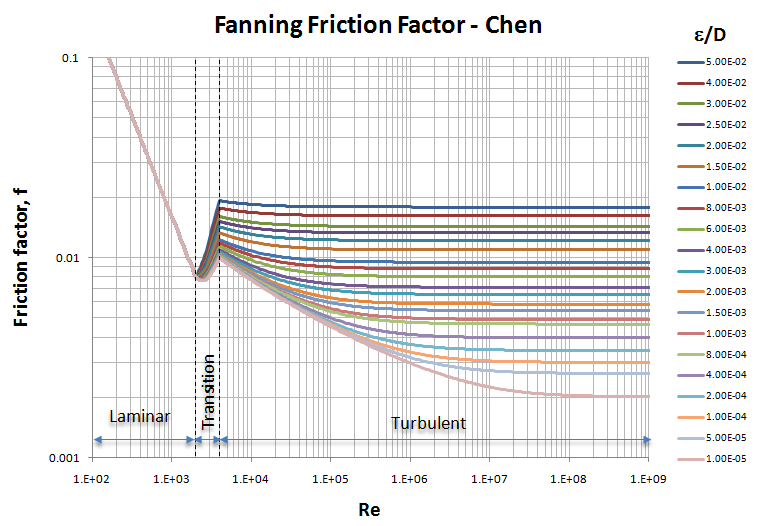
The friction factor in the transition from laminar to turbulent flow (2000<Re<4000) is approximated using the following expression:

Hydrostatic component

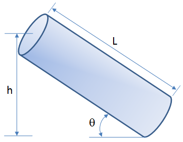
This component is of importance only when there are differences in elevation from the inlet end to the outlet end of a pipe segment. (In horizontal pipes this component is zero.) The hydrostatic pressure difference (ΔPHH) can be applied to all correlations simply by adding it to the friction component. The hydrostatic pressure drop (ΔPHH) is defined for a vertical pipe as follows:

A generalized form accounting for pipe inclination (using the angle with respect to the horizontal) can be written as:

Note:   To use the angle with respect to the vertical (for example, in well deviation surveys), change the trigonometric function to cosine.

For liquids, the density (ρ) is constant, and the above equation is easily evaluated.

For gases, density varies with pressure. Therefore, to evaluate the hydrostatic pressure loss or gain, the pipe (or wellbore) is subdivided into a sufficient number of segments, such that the density in each segment can be assumed to be constant. Note that this is equivalent to a Multi-Step Cullender and Smith calculation.

Flow correlations

Many single-phase correlations exist that were derived for different operating conditions or from laboratory experiments. Generally speaking, these only account for the friction component (that is, they are applicable to horizontal flow). Typical examples are:

• Fanning gas (also known as Multi-Step Cullender and Smith when applied to wellbores)
• Fanning liquid

In Harmony™, for cases that involve a single phase, the Gray, Hagedorn and Brown, Beggs and Brill and Petalas and Aziz methods revert to the Fanning single-phase correlations. For example, if the Gray correlation was selected, but there was only gas in the system, the Fanning gas correlation is used.

Note:   Single-phase correlations can be used for vertical or inclined flow provided that the hydrostatic pressure drop is accounted for in addition to the friction component. Even though a particular correlation may have been developed for flow in a horizontal pipe, incorporation of the hydrostatic pressure drop allows the correlation to be used for flow in a vertical pipe. This adaptation is rigorous, and has been implemented into all of the correlations used in Harmony™. Nevertheless, for identification purposes, the correlation’s name has been left unchanged.

Multiphase flow

Multiphase pressure loss calculations parallel single-phase pressure loss calculations. Essentially, each multiphase correlation makes its own specific modifications to the hydrostatic pressure difference and the friction pressure loss calculations, in order to make them applicable to multiphase situations.

The presence of multiple phases greatly complicates pressure drop calculations. This is due to the fact that the properties of each fluid present must be taken into account. Also, the interactions between each phase must be considered. Mixture properties must be used, and therefore the gas and liquid in-situ volume fractions throughout the pipe need to be determined. In general, multiphase correlations are essentially two-phase, and not three-phase. Accordingly, the oil and water phases are combined, and treated as a pseudo single-liquid phase, while gas is considered a separate phase.

The hydrostatic pressure difference calculation is modified by defining a mixture density. This is determined by a calculation of in-situ liquid holdup (amount of liquid in the pipe section). Some correlations determine holdup based on defined flow patterns.

The friction pressure loss is modified in several ways by adjusting the friction factor (f), the density (ρ), and velocity (v) to account for multiphase mixture properties.

The multiphase pressure loss correlations in Harmony™ are based on the Fanning friction pressure loss equation. They can be grouped as follows:

Do not account for flow patterns:

• Gray — Developed using data from gas and condensate wells.
• Hagedorn and Brown — Derived using a test well running different oils and air

Consider flow patterns:

• Beggs and Brill — Correlation derived from experimental data for vertical, horizontal, inclined uphill, and downhill flow of gas-water mixtures
• Petalas and Aziz — Mechanistic model combined with empirical correlations. This multi-purpose correlation is applicable for all pipe geometries, inclinations, and fluid properties.

These models can be used for gas-liquid multiphase flow, single-phase gas, or single-phase liquid, because in single-phase mode, they revert back to the Fanning equation, which is equally applicable to either gas or liquid.

Note:   The Gray and Hagedorn and Brown correlations were derived for vertical wells and may not apply to horizontal pipes.

Flow fluid properties

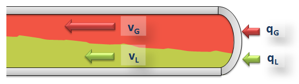
Superficial Velocities

The superficial velocity of each phase is defined as the volumetric flow rate of the phase divided by the cross-sectional area of the pipe (as though that phase alone was flowing through the pipe). Therefore:

Since the liquid phase accounts for both oil and water:

QL = QOBO + (QW– QWCQG)BW

and the gas phase accounts for the solution gas going in and out of the oil as a function of pressure:

QG = QG – QORS

the superficial velocities can be rewritten as:

The oil, water, and gas formation volume factors (BO, BW, and Bg) are used to convert the flow rates from standard (or stock tank) conditions to the prevailing pressure and temperature conditions in the pipe.

Since the actual cross-sectional area occupied by each phase is less than the cross-sectional area of the entire pipe, the superficial velocity is always less than the true in-situ velocity of each phase.

Mixture velocity

Mixture velocity is another parameter that is often used in multiphase flow correlations. The mixture velocity is given by:

vm = vsL + vsG

Slippage and the liquid holdup effect

When two or more phases are present in a pipe, they tend to flow at different in-situ velocities. These in-situ velocities depend on the density and viscosity of each phase. Typically the phase that is less dense flows faster than the other. This causes a "slip" effect between the phases. As a consequence, the in-situ volume fractions of each phase (under flowing conditions) differ from the input volume fractions of the pipe.

If the slip condition is omitted, the in-situ volume fraction of each phase is equal to the input volume fraction.

In-situ volume fraction (liquid holdup with slip)

The in-situ volume fraction, EL (or HL), is often the value that is estimated by multiphase correlations. Because of slippage between phases, the liquid holdup (EL) can be significantly different from the input liquid fraction (CL). In other words, the liquid slip holdup (EL) is the fraction of the pipe that is filled with liquid when the phases are flowing at different velocities. It can be defined as follows:

Input volume fraction (no-slip holdup)

The input volume fractions are defined as:

We can also write them as a function of the superficial velocities as:

Note:   QL is the liquid rate at the prevailing pressure and temperature. Similarly, QGBg is the gas rate at the prevailing pressure and temperature.

The input volume fractions, CL and EL, are known quantities, and are often used as correlating variables in empirical multiphase correlations. In the event that slip effects are neglected (gas and liquid traveling at the same velocity), the in-situ liquid fraction is equal to the input liquid fraction (EL = CL).

Actual velocities

Once the liquid holdup has been determined, the actual velocities for each phase can be determined as follows:

Density

Density (ρ) is used in hydrostatic pressure difference calculations. The method for calculating ρ depends on whether flow is compressible or incompressible (multiphase or single-phase). For multiphase flow, the calculations become even more complicated than for single-phase flow because ρ is calculated from the in-situ mixture density, which in turn is calculated from the "liquid holdup." The liquid holdup, or in-situ liquid volume fraction, is obtained from one of the multiphase flow correlations, and depends on several parameters including the gas and liquid rates and the pipe diameter. Note that this is in contrast to the way density is calculated for friction pressure loss.

Mixture density

Mixture density is a measure of the in-situ density of the mixture, and is defined as follows:

ρm = ρLEL + ρGEG = ρLEL + ρG(1 – EL)

Note:   Mixture density is defined in terms of in-situ volume fractions (EL), whereas no-slip density is defined in terms of the input volume fractions (CL).

No-slip density

"No-slip" density is the density that is calculated with the assumption that both phases are moving at the same in-situ velocity. No-slip density is therefore defined as follows:

ρNS = ρLCL + ρGCG = ρLCL + ρG(1 – CL)

Note:   No-slip density is defined in terms of the input volume fractions (CL), whereas the mixture density is defined in terms of the in-situ volume fractions (EL).

Mixture viscosity

Mixture viscosity is a measure of the in-situ viscosity of the mixture and can be defined in several different ways. In general, unless otherwise specified, is defined as follows:

μm = μLEL + μG EG = μL EL + μG (1 – EL)

Note:   Mixture viscosity is defined in terms of in-situ volume fractions (EL), whereas no-slip viscosity is defined in terms of input volume fractions (CL).

No-slip viscosity

"No-slip" viscosity is the viscosity that is calculated with the assumption that both phases are moving at the same in-situ velocity. There are several definitions of "no-slip" viscosity. In general, unless otherwise specified, µNS is defined as follows:

μNS = μL CL + μG CG = μL CL + μG (1 – CL)

Surface tension

The surface tension (interfacial tension) between the gas and liquid phases has very little effect on two-phase pressure drop calculations. However, a value is required for calculating certain dimensionless numbers used in some of the pressure drop correlations. Empirical relationships for estimating the gas / oil interfacial tension and the gas / water interfacial tension were presented by Baker and Swerdloff, Hough and by Beggs.

Gas / oil interfacial tension

The dead oil interfacial tension at temperatures of 68°F and 100°F is given by:

σ68 = 39 – 0.2571 (API)

σ100 = 37.5 – 0.2571 (API)

If the temperature is greater than 100°F, the value at 100°F is used. If the temperature is less than 68°F, the value at 68°F is used. For intermediate temperatures, linear interpolation is used.

As pressure is increased and gas goes into solution, the gas / oil interfacial tension is reduced. The dead oil interfacial tension is corrected for this by multiplying by a correction factor:

C = 1.0 – 0.024P0.45

The interfacial tension becomes zero at miscibility pressure, and for most systems this is at any pressure greater than about 5000 psia. After the correction factor becomes zero (at about 3977 psia), 1 dyne/cm is used for calculations.

Gas / water interfacial tension

The gas / water interfacial tension at temperatures of 74°F and 280°F is given by:

σW(74) = 75 – 1.108P0.349

σW(280) = 53 – 0.1048P0.637

If the temperature is greater than 280°F, the value at 280°F is used. If the temperature is less than 74°F, the value at 74°F is used. For intermediate temperatures, linear interpolation is used.

Friction component

In pipe flow, friction pressure loss is the component of total pressure loss caused by viscous shear effects. Friction pressure loss always acts against the direction of flow. It is combined with the hydrostatic pressure difference (which may be positive or negative, depending on whether the flow is upward (also known as uphill) or downward (downhill)) to give the total pressure loss.

Friction pressure loss is calculated from the Fanning friction factor equation as follows:

In the above equation, the variables f, ρ, and v are treated differently by each correlation.

Each multiphase flow correlation finds the friction factor differently. This calculation depends, in part, on the gas and liquid flow rates, but also on the standard Fanning (single-phase) friction factor chart. When evaluating the Fanning friction factor, there are many ways of calculating the Reynolds number depending on how the density, viscosity, and velocity of the two-phase mixture are defined. For example, the Beggs and Brill calculation of the Reynolds number uses mixture properties that are calculated by prorating the property of each individual phase in the ratio of the input volume fraction (and not of the in-situ volume fraction).

Hydrostatic component

Hydrostatic pressure difference is the component of pressure loss (or gain) attributed to the earth’s gravitational effect. It is of importance only when there are differences in elevation from the inlet end to the outlet end of a pipe segment. This pressure difference can be positive or negative depending on the reference point (inlet higher vertically than outlet, or outlet higher than inlet). Under ALL circumstances, regardless of what sign convention is used, the contribution of the hydrostatic pressure calculation must be such that it tends to make the pressure at the vertically-lower end higher than that at the upper end.

The hydrostatic pressure difference is calculated as follows:

In the equation above, the problem lies in finding an appropriate value for density, as discussed below:

• For a single-phase liquid, the density of the mixture is equal to the liquid density.
• For a single-phase gas, density varies with pressure, and the calculation must be done sequentially in small steps to allow density to vary with pressure.
• For multiphase flow, density is calculated from the in-situ mixture density, which in turn is calculated from the liquid holdup. The liquid holdup is obtained from multiphase flow correlations, such as Beggs and Brill, and depends on the gas and liquid rates, pipe diameter, etc.
• For a horizontal pipe segment, θ = 0.0, and there is NO hydrostatic pressure loss.

Flow correlations

Many of the published multiphase flow correlations are applicable for vertical flow only, while others apply for horizontal flow only. Other than the Beggs and Brill correlation and the Petalas and Aziz mechanistic model, there are not many correlations that were developed for the whole spectrum of flow situations that can be encountered in oil and gas operations — namely, uphill, downhill, horizontal, inclined, and vertical flow. However, we have adapted all of the correlations (as appropriate) so that they apply to all flow situations. This includes these multiphase flow correlations:

• Beggs and Brill — one of the few published correlations capable of handling all of the flow directions. It was developed using sections of pipeline that could be inclined at any angle.
• Gray — developed for vertical flow in wet gas wells. We have modified it, so that it applies to flow in all directions by calculating the hydrostatic pressure difference using only the vertical elevation of the pipeline segment, and the friction pressure loss based on the total length of the pipeline.
• Hagedorn and Brown — developed for vertical flow in oil wells. We have modified it, so that it applies to flow in all directions by calculating the hydrostatic pressure difference using only the vertical elevation of the pipe segment, and the friction pressure loss based on the total pipeline length.
• Petalas and Aziz — developed to overcome the limitations imposed by using previous correlations. It applies to all pipe geometries, fluid properties, and flow in all directions. A mechanistic approach is combined with empirical closure relationships to provide a model that is more robust than other models and can be to used predict pressure drop and holdup in pipes over a more extensive range of conditions.

Each of these correlations was developed for its own unique set of experimental conditions, or designed using a mechanistic modeling approach, and accordingly, results vary between them.

For multiphase flow in essentially vertical wells, the available correlations are Beggs and Brill, Petalas and Aziz, Gray and Hagedorn and Brown. If used for single-phase flow, these four correlations devolve to the Fanning gas or Fanning liquid correlation as needed.

When creating a new wellbore, Harmony sets a default multiphase correlation depending upon the type of well that exists in the Entity Viewer. This default correlation is based on our expected use cases, and thus may not apply to every wellbore. Of course, the correlation for the wellbore configuration can be changed at any time.

Note:   The Gray and Hagedorn and Brown correlations were derived for vertical wells and may not apply to horizontal pipes. In Harmony, the Gray, the Hagedorn and Brown, the Beggs and Brill, and the Petalas and Aziz models revert to the appropriate single-phase Fanning correlation (Fanning liquid or Fanning gas).

Beggs and Brill correlation

The Beggs and Brill (1973) correlation is one of the few published correlations capable of handling all these flow directions. It was developed measuring the flow of water and air through 1" and 1-1/2" sections of acrylic pipe that could be inclined at different angles from the horizontal.

The Beggs and Brill multiphase correlation deals with both friction pressure loss and hydrostatic pressure difference. First, the corresponding flow pattern for the particular combination of gas and liquid rates (segregated, intermittent, or distributed) is determined. The liquid holdup, and hence, the in-situ density of the gas-liquid mixture, is then calculated according to the identified flow pattern to obtain the hydrostatic pressure difference. A two-phase friction factor is calculated based on the input gas-liquid ratio and the Fanning friction factor. From this, friction pressure loss is calculated using input gas-liquid mixture properties.

In our implementation, whenever single-phase flow is encountered during pressure loss calculations, the Beggs and Brill correlation devolves to the Fanning gas or Fanning liquid correlation.

Flow pattern map

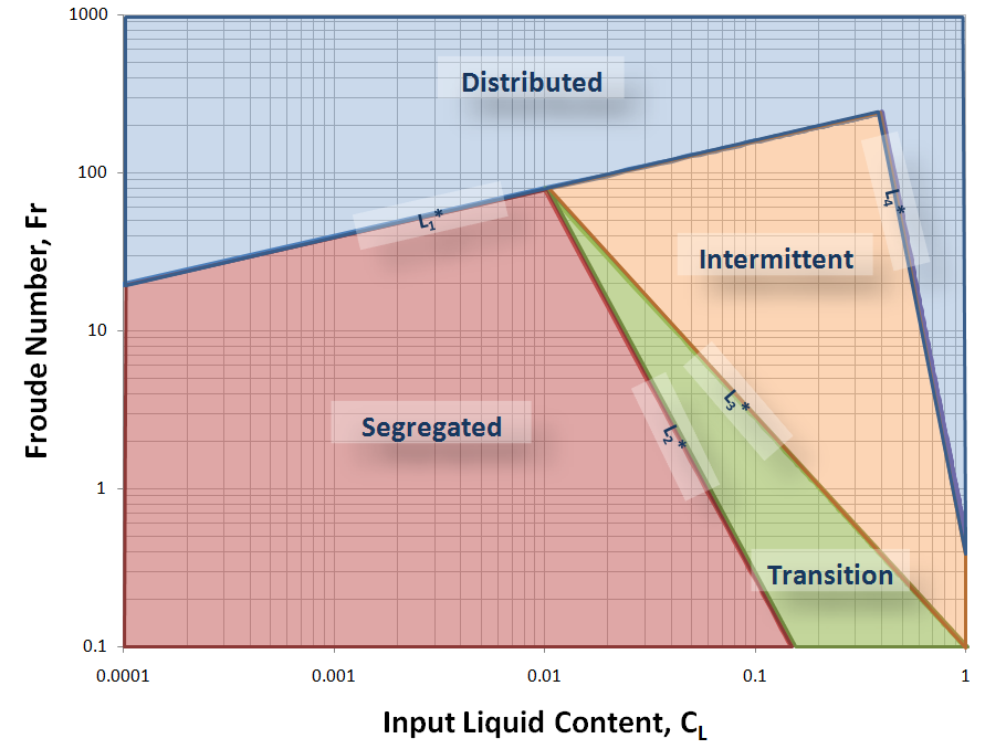
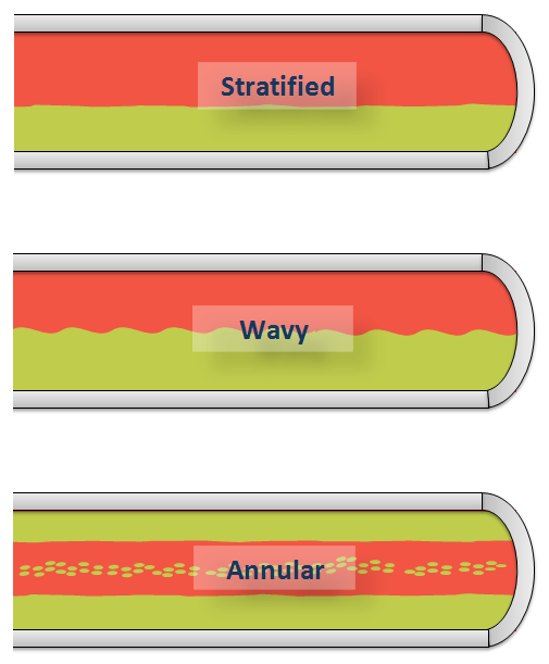
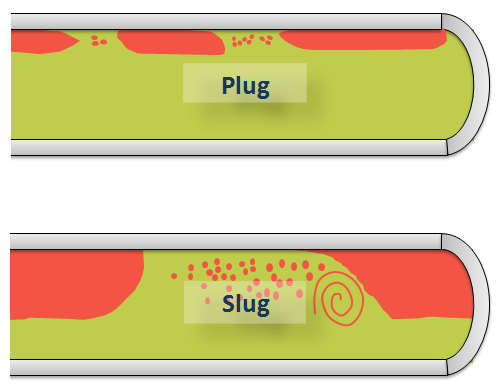
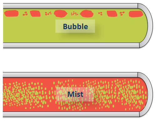
Unlike the Gray or Hagedorn and Brown correlations, the Beggs and Brill correlation needs to identify the flow pattern at the given flowing conditions in order to calculate the liquid holdup and friction. For this purpose, the Beggs and Brill correlation makes use of a horizontal flow-pattern map built based on the Froude number of the mixture (Frm)  and input liquid content (no-slip liquid holdup, CL).

In order to build the flow map, the observed flow patterns were grouped as: segregated (stratified, wavy, and annular flow), intermittent (plug and slug flow), distributed (bubble and mist flow), and transition (flow pattern included after a modification of the original publication that considers the region between the segregated and intermittent grouped patterns).

The boundaries between these groups of flow patterns appear as curves in a log-log plot in the original publication by Beggs and Brill. This was later revised so that straight lines could be used instead. We use this modified flow-pattern map in our calculations. The revised lines that define the boundaries are defined as follows (where * stands for the modification of the original curve to a straight line in a log-log plot):

The identified flow pattern is the one that would exist if the pipe were horizontal. Unless the pipe is actually in the horizontal position, the Beggs and Brill correlation is not able to recognize the actual flow pattern under the given conditions. Therefore, to calculate the liquid holdup, we first determine the liquid holdup for the horizontal flow, and this value is then corrected for the angle of interest.

The Froude number is a dimensionless number that relates the inertia with respect to the gravitational forces. For a mixture, it can be obtained by:

Once the input liquid content (CL) and Froude number of the mixture (Frm) are determined, the corresponding flow pattern is identified when the following inequalities are satisfied.

Segregated

if

or

Intermittent

if

or

Distributed

if

or

Transition

if

Hydrostatic Pressure Difference

Once the flow pattern has been determined, the liquid holdup is then calculated. Beggs and Brill divided the liquid holdup calculation into two parts. First, the liquid holdup for horizontal flow, EL(0), is determined. Afterward, this horizontal holdup is corrected for inclined flow to obtain the actual holdup, EL(θ). The horizontal holdup must be EL(0) ≥ CL. Therefore, in the event that EL(0) < CL, the horizontal holdup is set to EL(0) = CL. The expression used to calculate the horizontal holdup changes per flow pattern group as follows:

Segregated

Intermittent

Distributed

Transition

E_L(0)_transition = A E_L(0)_segregated + B E_L(0)_intermittent

where:

B = 1 – A

Once the horizontal in-situ liquid volume fraction is determined, the actual liquid volume fraction is obtained by correcting EL(0) by an inclination factor B(θ):

where:

β is a function of the flow pattern and is also related to the direction of inclination of the pipe (uphill or downhill flow).

For uphill flow

1. Segregated

1. Intermittent

Distributed

β = 0

For downhill flow

1. ALL flow pattern groups

where Frm is the Froude number of the mixture and NLv is the liquid velocity number given by:

Note:   β must always be ≥ 0. Therefore, if a negative value is calculated for β, β = 0.

Once the actual liquid holdup EL(θ) is calculated, the mixture density ρm is obtained. Mixture density, in turn, is used to calculate the pressure change due to the hydrostatic head of the vertical component of the pipe or well.

Beggs and Brill - Friction Pressure Loss

In order to calculate frictional losses, a normalizing friction factor (fNS) is used. To determine fNS, we use the Fanning friction factor calculated using the Chen equation. For this purpose, the no-slip Reynolds number is used:

Based on experimental data, Beggs and Brill presented a correlation for the ratio of the two-phase friction factor (ftp) and the normalizing (no-slip) friction factor resulting in the following exponential equation:

The value of S depends on the no-slip and the actual liquid holdup:

where:

Severe instabilities have been observed when the equation for S is used as published. To solve for them, the following considerations are used:

• If y = 0, then S=0 (to ensure that the expression is reduced to single-phase liquid)
• If 1 < y < 1.2, then S = ln(2.2y – 1.2)

After a valid value for S has been found, you can solve for the two- phase friction factor:

ftp = fNSes

Finally, the expression for pressure loss due to friction is:

Gray Correlation

The Gray correlation was developed by H.E. Gray (1978) specifically for wet gas wells. Although this correlation was developed for vertical flow, we have implemented it to be used in both vertical and inclined pipe pressure-drop calculations. To correct pressure drop for situations with a horizontal component, the hydrostatic head has only been applied to the vertical component of the pipe, while friction is applied to the entire length of pipe.

First, the in-situ liquid volume fraction is calculated. The in-situ liquid volume fraction is then used to calculate mixture density, which in turn is used to calculate the hydrostatic pressure difference. The input gas-liquid mixture properties are used to calculate an effective roughness of the pipe. This effective roughness is then used in conjunction with a constant Reynolds number of 10⁷ to calculate the Fanning friction factor. The pressure difference due to friction is calculated using the Fanning friction pressure-loss equation.

Gray – Hydrostatic Pressure Difference

The Gray correlation uses three dimensionless numbers in combination to predict the in-situ liquid volume fraction. These three dimensionless numbers are:

where:

The dimensionless numbers are then combined as follows:

where:

Once the liquid holdup (EL) is calculated, it is used to obtain the mixture density (ρm). Mixture density, in turn, is used to compute the pressure change due to the hydrostatic head of the vertical component of the pipe.

Gray – Friction Pressure Loss

The Gray Correlation assumes that the effective (also known as apparent) roughness of the pipe (ke) is dependent on the value of Rv. The conditions are as follows:

If Rv ≥ 0.007 then:

ke = k°

if Rv < 0.007 then:

where:

and k is the absolute roughness of the pipe (single-phase dry gas flow). The resulting effective roughness (ke) must be larger than or equal to 2.77×10-5.

The relative roughness of the pipe is then calculated by dividing the effective roughness by the diameter of the pipe. The Fanning friction factor is obtained using the Chen equation and assumes a Reynolds number of 107. Finally, the expression for the friction pressure loss is:

Note:   The original publication contains a misprint in the calculation of ke: the constant should be 0.007 instead of 0.0007. We include this correction in our calculations. Additionally, the volume of water condensation is estimated using Bukacek’s correlation (including the corrections by McKetta and Wehe) and is considered in the pressure-drop calculations.

Hagedorn and Brown

Experimental data obtained from a 1500 ft deep instrumented vertical test well was used in the development of the Hagedorn and Brown correlation. Pressures were measured for flow in tubing sizes of 1 ", 1 ¼” and 1 ½" OD. A wide range of liquid rates and gas / liquid ratios were used. As with the Gray correlation, our software calculates pressure drops for horizontal and inclined flow using the Hagedorn and Brown correlation, although the correlation was developed strictly for vertical wells. The software uses only the vertical depth to calculate pressure loss due to hydrostatic head, and the entire pipe length to calculate friction.

The Hagedorn and Brown method has been modified for the bubble flow regime (Economides et al, 1994). If bubble flow exists, the Griffith correlation is used to calculate the in-situ volume fraction. In such cases, the Griffith correlation is also used to calculate pressure drop due to friction. If bubble flow does not exist, then the original Hagedorn and Brown correlation is used to calculate the in-situ liquid volume fraction. Once the in-situ volume fraction is determined, it is compared with the input volume fraction. If the in-situ volume fraction is smaller than the input volume fraction, the in-situ fraction is set to equal the input fraction (EL = CL). Next, the mixture density is calculated using the in-situ volume fraction and used to calculate the hydrostatic pressure difference. The pressure difference due to friction is calculated using a combination of in-situ and input gas-liquid mixture properties.

Hagedorn and Brown - Hydrostatic Pressure Difference

The Hagedorn and Brown correlation uses four dimensionless parameters (based on the work of Duns and Ros) to correlate liquid holdup. These four parameters are:

The method of calculation is based on the use of several plots where various combinations of these parameters are calculated and plotted against some correlated terms to determine the liquid holdup. For programming purposes, these curves were discretized into equations.

The first curve provides a value for a dimensionless parameter called NLC, which is correlated with the dimensionless number NLL. Therefore, once NL is calculated, it is possible to obtain NLC from the following plot:

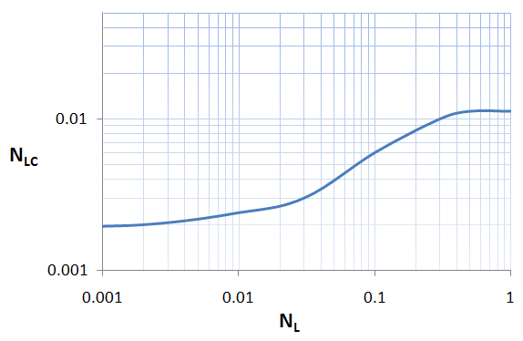
The value of NLC is then used to calculate the dimensionless number, :

The next plot contains a curve correlating the liquid holdup divided by a correction factor (EL / Ψ) against the dimensionless group, . After  is calculated, you can then find the value of EL / Ψ by making use of the following plot:

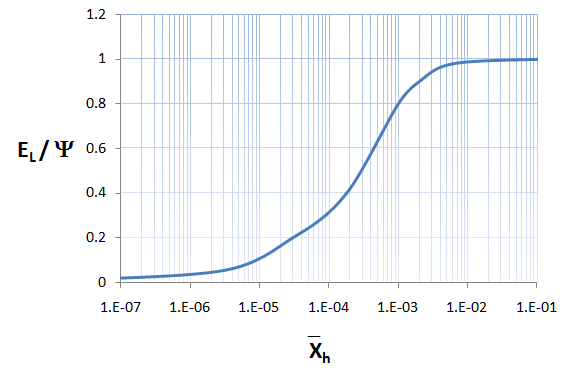
Finally, the third curve correlates the correction factor Ψ with the dimensionless number, :

A typical discretized curve to find Ψ can be as follows:

After finding Ψ, the in-situ liquid volume fraction (EL) can be calculated taking the previously found EL / Ψ:

We have implemented a correction to replace the liquid holdup value with the "no-slip" (input) liquid volume fraction, if the calculated liquid holdup is less than the no-slip liquid volume fraction:

if EL < CL, then EL = CL

After finding EL, the hydrostatic head is calculated by the standard equation:

where:

ρm = ρL  EL + ρG (1 – EL)

Hagedorn and Brown - Friction Pressure Loss

The friction factor is calculated using the Chen equation using a Reynolds number equal to:

Note:   In the Hagedorn and Brown correlation, mixture viscosity is given by:

The pressure loss due to friction is then given by:

where:

Modification to the Hagedorn and Brown Correlation: the Griffith Correlation for Bubble Flow

The Hagedorn and Brown correlation makes use of the Griffith correlation (1961) for the bubble flow regime. Bubble flow exists if CG < LB, where:

If the calculated value of LB is less than 0.13, then LB is set to 0.13. If the flow regime is found to be bubble flow, then the Griffith correlation is applied. Otherwise, the original Hagedorn and Brown correlation is used.

In the Griffith correlation, liquid holdup is given by:

Griffith suggested a constant value of vs = 0.8 ft/s as a good average value, which is the one considered in our calculations.

The true in-situ liquid velocity is given by:

The hydrostatic head is then calculated the standard way.

The pressure drop due to friction is also affected by the use of the Griffith correlation because EL enters into the calculation of the Reynolds number via the in-situ liquid velocity. The Reynolds number is calculated using the following format:

The single-phase liquid density, in-situ liquid velocity, and liquid viscosity are used to calculate the Reynolds number. This is unlike the majority of multiphase correlations, which usually define the Reynolds number in terms of mixture properties rather than single-phase liquid properties. The Reynolds number is used to calculate the friction factor using the Chen equation. The liquid density and the in-situ liquid velocity are then used to calculate the pressure drop due to friction:

Petalas and Aziz Mechanistic Model

The Petalas and Aziz mechanistic model (2000) was not built for a specific set of data or fluid properties. Instead, the authors applied first principles to the possible flow patterns that can be observed at different inclinations. For this reason, it is applicable to any pipe inclination and fluid properties. The model is a refinement of a previous study by the authors (1996) where subsets of a database of over 20,000 laboratory measurements and data from approximately 1,800 wells were used.

The method could be summarized as follows:

• Assume the existence of a flow pattern
• Evaluate if this flow pattern is stable:

• If the check fails, go back and select another flow pattern
• If stable conditions are met, go ahead with the calculation of liquid holdup and the friction factor

• Calculate pressure losses using the found values for the friction factor and liquid holdup

With the continuous evaluation of the stability of the flow patterns, you can create the corresponding flow-pattern map to the given flowing conditions. This screenshot shows a typical flow-pattern map for vertical upward gas-oil flow:

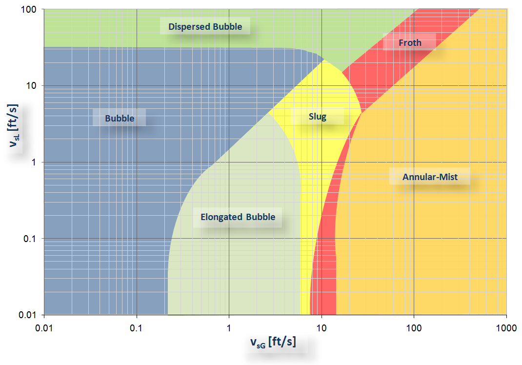
Flow Pattern Map

Dispersed Bubble flow

In order to have dispersed bubble flow, two requirements must be fulfilled.

The first criterion is based on Barnea’s transition from dispersed to slug flow while using the slug liquid holdup calculation based on Gregory et al:

where:

vm = vsG + vsL

Also, to be able to sustain dispersed bubble flow, the ratio of the superficial gas velocity with respect to the mixture velocity should be:

Stratified Flow

The consideration here is that stratified flow can be possible only in downward (downhill) or horizontal flow. A momentum balance is obtained based on the one proposed by Taitel and Dukler. The first step consists in calculating (dimensionless liquid height) by solving:

where:

and

fG is obtained from standard methods where:

where the hydraulic diameter of the gas phase, DG, is obtained by:

fL from:

where fsL is a friction factor based on the superficial velocity, which is calculated from standard methods using the pipe roughness and the Reynolds number:

fi from:

using a liquid Froude number defined as:

use Lockhart-Martinelli parameters:

X2 F2 – F1 – 4Y = 0

where:

where:

with the geometric variables:

Solve for hL / D iteratively. Afterwards, we verify that stratified flow exists if:

and if:

Note:   When cosθ ≤ 0.02, then, cosθ = 0.02.

To distinguish between stratified smooth and stratified wavy flow regimes:

stratified smooth flow exists if:

where s=0.06, and if:

Annular-Mist Flow

Calculate the dimensionless liquid film thickness ( ), making the momentum balance on the liquid film and gas core with liquid droplets:

Annular-mist flow exists if:

where is determined from the following equations:

Solve for  iteratively.

Bubble Flow

Bubble flow exists if:

and if:

where:

C1 = 0.8

γ = 1.3

db = 7mm

with:

Also, transition to bubble flow from intermittent flow occurs when:

EL > 0.25

where:

Intermittent Flow

Note:   The intermittent flow model used here includes slug and elongated bubble flow regimes.

Intermittent flow exists if:

EL > 0.24

where:

If EL > 1, then EL = CL.

and if:

where:

vm = vsL + vsG

• If ELL > 0.24 and ELs < 0.9, then slug flow
• If EL > 0.24 and ELs > 0.9, then elongated bubble flow

Froth Flow

If none of the transition criteria for intermittent flow are met, the flow pattern is then designated as froth. Froth flow implies a transitional state between the other flow regimes.