Fractional Dimension Rate Transient Analysis (FD-RTA)

Introduction for Classical RTA vs FD-RTA (for horizontal multi-frac wells)

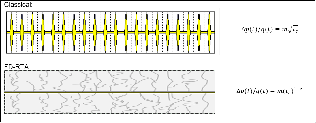
The Classical way to analyse production from Horizontal Multi-frac wells assumes that fractures are distributed uniformly along the wellbore. In this case, the well experiences linear flow (perpendicular to the fractures) until the transient reaches the boundaries of the SRV. The analysis in this case is based on the fact that linear flow behaviour can be approximated by:

Equation 1

Where t_c is material balance time.

However, for some Horizontal Multi-frac wells fracture distribution is not uniform. As a result, production data does not exhibit linear behaviour. Instead, it follows Equation 2 below during the (characteristic) flow within SRV. (Note: in this case early data follows a straight line on the log-log plot, and the slope of this line is equal to 1-δ).

Equation 2

Where δ is a flow dimension parameter.

Fractional Dimension RTA (FD-RTA) is used to analyse, history-match and forecast wells exhibiting such behaviour.

Create FD-RTA Analysis

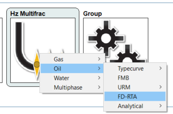
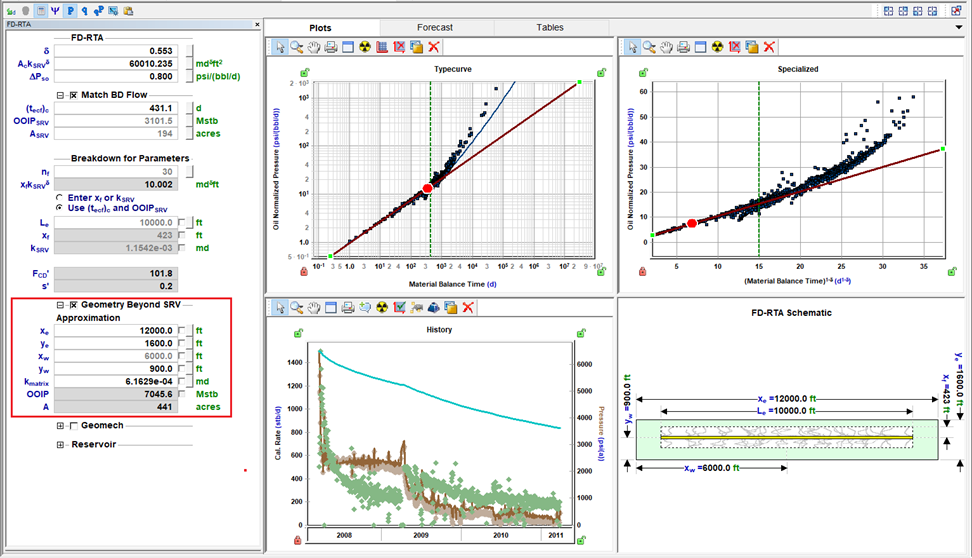
The Fractional Dimension Rate Transient Analysis (FD-RTA) worksheet is accessible by clicking the Hz Multifrac thumbnail.

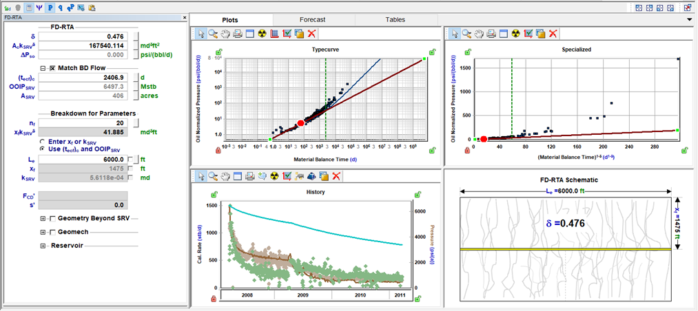
In a newly created worksheet, the input values in the parameter pane are populated by default, and resulting datasets can be seen on the Typecurve and Specialized plots.

Performing FD-RTA is accomplished by changing those input values. This can be done by typing new values, manipulating analysis lines or by using Automatic Parameter Estimation (APE). This is described in more detail in subsequent sections.

Plots

FD-RTA consists of two analysis plots, one History plot and a FD-RTA Schematic.

During data analysis, it is recommended to look at all 3 plots simultaneously. Moving the interactive line on any of the plots will update the lines on the other plots accordingly, and calculated datasets displayed on the History plot will also be updated. Once the analysis is completed, you should expect to observe a good match to the data on all 3 plots.

If AutoCalc () mode is enabled, all calculation results will be updated automatically every time interactive lines are moved or input values are changed on the parameters pane. If AutoCalc mode is off, you will need to use the Synthesize () function to see the updated calculated results.

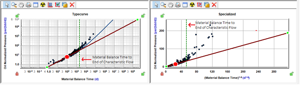
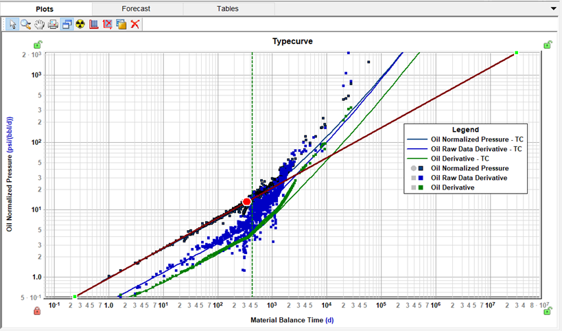
Interactive Typecurve Plot

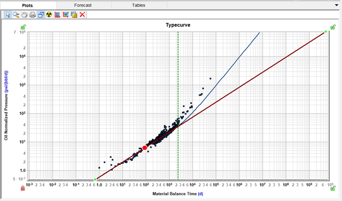
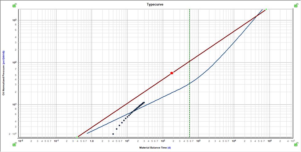
This is a log-log plot, that displays the following:

• Data points (dark blue points): these represent normalized pressure vs. material balance time (or pseudo-time).

• Analysis line (brown line): This is an interactive straight line, where the slope of the line is (1-δ) and its vertical position is related to the value of the CFP (characteristic flow parameter) A_ck_SRV^δ.

• End of characteristic flow line (dashed green line): This is an interactive vertical line positioned at (t_ecf)_c. Note that the value is in terms of material balance time.

• Typecurve (dark blue line): The Typecurve corresponds to the parameters given in the input grid. This curve follows the Analysis line until (t_ecf)_c, at which point the transient reaches the boundary of the SRV region. From there, the Typecurve transitions from characteristic flow towards boundary-dominated flow.

If ‘Geometry Beyond SRV’ is checked, the Typecurve behaviour is slightly different, for more details, refer to Modeling reservoir beyond SRV.

• Raw Data Derivative (blue points and lines) – can be displayed from FD-RTA Options dialog ( ). For more details, refer to Derivatives section of this chapter.

• Derivative (green points and lines) – can be displayed from FD-RTA Options dialog ( ). For more details, refer to Derivatives section of this chapter.

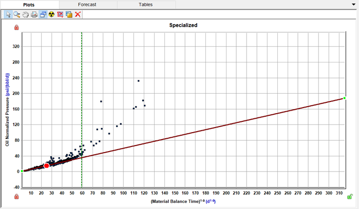
Specialized Plot

The Specialized Plot displays normalized pressure vs. (material balance time)^1-δ. The first portion of the data corresponds to the flow within the SRV. FD-RTA assumes that the flow within SRV follows Equation 2; therefore, the first portion of the data should exhibit a straight line with a slope of ‘m’ and an intercept of ∆P_s (delta pressure due to skin). Note that ‘m’ is inversely proportional to the characteristic flow parameter A_ck^SRVδ.

This plot displays the following:

• Data points (blue points): Representing normalized pressure vs. (material balance time)^1-δ

• Analysis line (brown line): An interactive straight line with the slope of ‘m’ and intercept of ∆P_s (delta pressure due to skin).

• End of characteristic flow line (dashed green line): An interactive vertical line positioned at (t_ecf)_c. Note that the value is in terms of material balance time.

The dashed green line in both the Typecurve plot and the Specialized plot are linked, they both represent the End of characteristic flow.

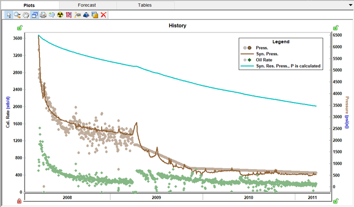
History Plot

Parameters given in the input grid (δ, CFP= A_ck_SRV^δ , ∆P_s and (t_ecf)_c) define the shape of the Typecurve displayed on the Typecurve plot. Essentially, this typecurve represents a constant rate solution for the system. (For more details, refer to the Fractional Dimension Rate Transient Analysis Theory (FD-RTA). The superposition of this typecurve with the historical production of the well gives calculated flowing pressures (p_wf)_calc.

The plot shows the calculated flowing pressures (represented by the brown line) along with actual pressures (depicted as brown dots) on the History Plot.

The main objective of history matching is to closely replicate actual data (rates or pressures) by adjusting the calculated output through changing the parameters.

If the CalcP icon ( ) is selected, rates will be used to calculate pressures. The History plot will display data points for actual rate and pressure, calculated pressure and calculated reservoir pressure.

If the CalcR icon is selected ( ) pressures will be used to calculate rates. The History plot will display data points for actual rate and pressure, calculated rate, and calculated reservoir pressure.

If you click the CalcBoth icon ( ), both above calculations will be performed independently. The history plot will display data points for actual rate and pressure, calculated rate, calculated flowing pressure, and the calculated reservoir pressure based on the calculated pressures and rates.

Matching characteristic flow (flow within SRV)

The first portion of the data within the SRV will appear as a straight line on the Typecurve plot and the Specialized plot. The slope and position of these straight lines give the values of delta (δ) and A_ck_SRV^δ. These lines can be manipulated until a good match is identified in the Typecurve and the Specialized plots resulting in a good match on the SRV portion of the History plot.

Matching the end of characteristic flow

The dashed green line on the Typecurve and the Specialized plots represents the Material Balance time to end of characteristic flow. As mentioned earlier, the first portion of the data will follow a straight line on the Typecurve and Specialized plots and in some cases your data will start diverging from this straight line. If this is the case, place the green dashed line where the data starts deviating. The data points beyond the green dashed line represent the portion of the data after the transient has reached the boundary of the SRV.

While analyzing the data, the aim is to match the time when the data deviates from the straight line, as well as the behaviour after this divergence happens.

You may need to include Geometry beyond SRV to match the behavior after t_ecf.

Note that the value of t_ecf is directly related to the size of the SRV (A_SRV and OFIP_SRV). The larger the SRV the longer it takes to reach its boundaries.

In FD-RTA analyses you can enter any of these 3 parameters, and the other 2 parameters will be calculated based on the one entered.

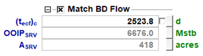
If the signature of the data is not pronounced enough to be able to uniquely identify the end of characteristic flow, you can check ‘Match BD Flow’ and enter OFIP_SRV or A_SRV if you know them from any external source.

If the well has not yet produced for a long enough time to reach the boundary of the SRV, you can enter A_SRV estimated based on analog wells and well spacing. Alternatively, you can uncheck ‘Match BD Flow’ option. In this case, history matching and forecast will be calculated assuming the data follows the same straight line (Equation 2) during the entire duration of history and forecast.

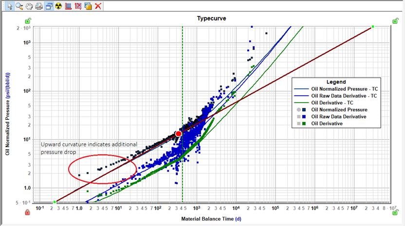
Accounting for additional pressure drop

Sometimes wells exhibit additional pressure drop, which may be due to damage around the fracture, cleanup, or other reasons. Parameter ∆P_s in Equation 2 accounts for this additional pressure drop.

When extra pressure drop due to skin is present, you may observe the early portion of the data curving upwards from the straight-line trend.

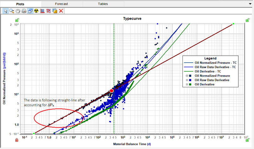
To account for the additional pressure drop, enter ∆P_s:

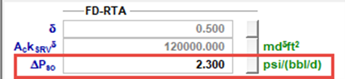
By doing this, the data points on the Typecurve plot are ‘corrected’ so that the data starts following the straight-line trend (with the same slope as the derivative).

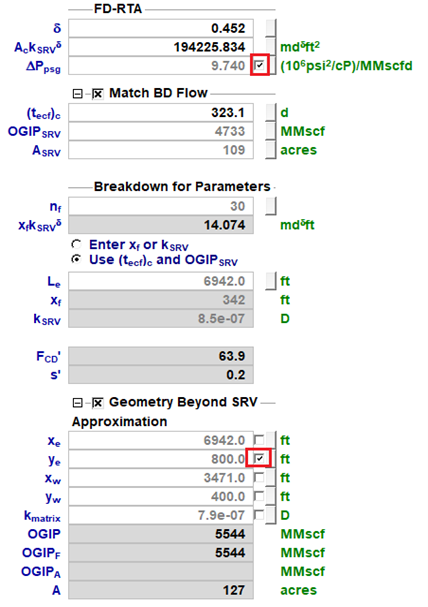
Breakdown for parameters

FD-RTA does not immediately provide values for individual completion parameters. Instead, the combined parameter of A_ck_SRV^δ is estimated from analyzing characteristic flow. Additionally, the SRV area (A_SRV) may be estimated from the position of the (t_efc)_c line. Individual parameters can be calculated assuming that other parameters are known.

Characteristic flow parameters can be broken down into completion parameters using one of the following methods:

• Select the option to ‘Use (t_ecf)_c | OFIP_SRV | A_SRV’ -

• Specify L_e (Effective Horizontal Well Length) and based on an estimated value of A_SRV, x_f will be calculated.

• Specify n_f (total number of fractures), k_SRV will be calculated based on x_f and CFP (A_ck_SRV^δ)

• Select the option to ‘Enter x_f or k_SRV’- if the data’s signature does not give a confident estimate for the exact (t_ecf)_c and A_SRV, enter either x_f or k_SRV, and the other parameter will be calculated based on the one you entered.

  All parameters under ‘Breakdown for Parameters’ are optional. You can use FD-RTA to estimate individual parameters (such as x_f, k_SRV), however, it is not required. History matching and forecasting can be performed without it.

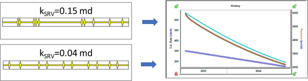
Non-uniqueness of k_SRV estimate

In case where fractures are distributed uniformly across the wellbore (δ=0.5), we can obtain a unique estimate for k_SRV based on A_ck_SRV^δ, if we provide values for x_f and n_f.

However, when fracture distribution is non-uniform, different combinations of fracture distributions and k_SRV may result in the same behavior. Therefore, the value of k_SRV is non-unique in such cases. In other words, when δ is not equal to 0.5, there is no way to calculate k_SRV (unless certain characteristics of the fracture distribution are known). k_SRV reported in the grid does not correspond to the actual permeability but represents the permeability of the proxy model that is used to generate the Typecurve. For cases when δ is close to 0.5, this estimate of permeability is close to the actual one, but for cases when δ is far from 0.5, permeability of the proxy model should not be used for reservoir characterization.

Modeling reservoir beyond SRV

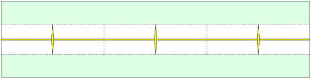
By default, it is considered that the boundary of the SRV is a no-flow boundary. However, we can account for the contribution from the matrix beyond SRV. To do so, check ‘Geometry Beyond SRV’ Option.

This option is only available when ‘Use (t_ecf)_c | OFIP_SRV | A_SRV’ is selected.

Once this option is checked, you can enter reservoir dimensions and k_matrix. The schematic will then reflect the additional area (matrix), and consequently, the match on the history plot will change, accounting for production from the matrix. This is particularly important for long-term forecasting.

Troubleshooting

FD-RTA calculation that includes ‘Geometry Beyond SRV’ follows the method proposed by Acuña, 2021. More details are provided here.

In short, the core of the method involves building the ‘investigated area’ function, denoted as A(r). This function describes the investigated area as a distance from the nearest fracture (r). Once this function is constructed, it is used to create a corresponding proxy model, that is then utilized to calculate the Typecurve and perform history-matching and forecast.

It is essential to note that building a one-dimensional function A(r) to accurately describe the transient propagation in a two-dimensional system may not always be possible. Therefore, calculations that include geometry beyond the SRV are approximate.

Below are a couple of examples where calculation may be inaccurate:

Example 1: Significant contribution from the matrix during the first characteristic flow.

Typically, the distance between fractures is much less than x_f. As a result, the transient reaches the boundaries of the SRV first, and then the contribution from the matrix becomes significant. However, if you set a small n_f, the contribution from beyond the SRV will start making effect before the transient reaches the end of the SRV.

As a result, you may notice that on the TypeCurve plot, the early portion of the data does not follow the analysis line. This discrepancy occurs because the position of the analysis line defines the contribution from the SRV. In this case, contribution from the matrix becomes significant even before the SRV is fully investigated, causing the typecurve to diverge from the analysis line.

If you observe such a behavior, evaluate if the values of n_f and x_f are reasonable and represent the actual geometry. You may consider increasing n_f (e.g. using number of fractures as oppose to number of fracture stages) and/or changing analysis parameters to increase x_f.

Example 2: Small delta

When the delta is very small (e.g. <0.25), it corresponds to the case when fracture distribution is very non-uniform. As a part of calculation flow, Harmony calculates the maximum distance between fractures (2r_SRV) corresponding to the given δ, k_SRV and (t_ecf)_c.

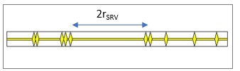
It is possible to set up the model in a way that that maximum distance becomes larger than Le. However, this set up does not reflect any realistic fracture distribution, and the calculation can’t be performed in this case (an error message will be displayed). In this case it is recommended to increase δ. If the data exhibits a steep slope (close to a unit slope), try to match this behaviour by decreasing (t_ecf)_c rather than decreasing δ.

 

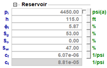
Reservoir

By default, FD-RTA uses the same reservoir parameters as are populated in Properties Editor for the well. However, you can change these values under Reservoir node:

Forecast

After the analysis have been performed, and you are happy with the history match seen on the History plot, you can create production forecasts under a variety of different constraints.

Please note that the forecast calculation is based of the same typecurve that is displayed on the Typecurve plot.

• If the ‘Match BD Flow’ checkbox is unchecked, the calculation will run assuming that the same characteristic flow will continue throughout.

• If ‘Match BD Flow’ checkbox is checked, and ‘Geometry Beyond SRV’ is unchecked, it will assume that the boundary of the SRV is a no-flow boundary. In other words, the calculation will assume characteristic flow (defined by δ) within the SRV, that transitions to a boundary-dominated flow. The time of transition is defined by A_SRV and (t_ecf)_c.

• If ‘Geometry Beyond SRV’ is checked, it will account for the contribution of the matrix. The calculation will assume characteristic flow (defined by δ) within the SRV, that transitions to a different flow regime that does not become boundary-dominated right away. The behavior after the end of characteristic flow is defined by the size of the reservoir beyond the SRV and by k_matrix.

Setting up the forecast is done similarly to how it’s done for Analytical models.

You can also Forecast using wellhead pressure.

Using derivatives

Derivatives can help identify signals that might not be very clear in the Typecurve plot, for example. They can also be used as a tool to help identify flow regimes.

It is possible to display the Raw Data Derivative and the Derivative on the Typecurve plot by clicking on the FD-RTA Options icon ( ).

The calculations used to calculate Raw Data Derivative and Derivative are the same as what is used in other analyses in Harmony. You can find details for those calculations here.

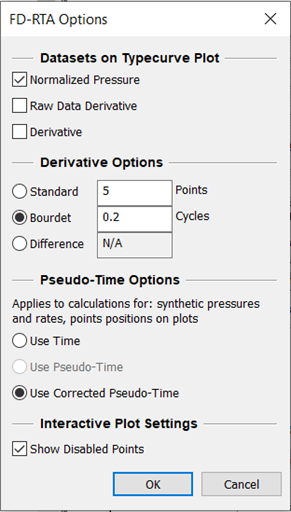
Options dialog box

The FD-RTA Options opens the FD-RTA Options dialog box, where you can check the datasets that you want to display on the Typecurve Plot, as well as change the default options for the way derivatives are calculated (Standard, Bourdet, or Difference). It also enables you to choose between using Time or Corrected Pseudo-Time when analyzing Gas wells. Also, you have the option to display your disabled points.

Adsorption

To consider the effect of adsorbed gas, click the Adsorption checkbox in the FD-RTA parameters pane. Note that this option is applicable only for Gas FD-RTA (not for Oil or Water FD-RTA).

For more information, see Langmuir isotherm.

After selecting Adsorption in the selection tree, the following properties are displayed:

• V_LS, P_LS — Langmuir volume and Langmuir pressure (for shale).

• ρ_b — bulk density (for shale).

You can also choose Ads. Sat. (adsorption saturation correction) in the selection tree, with the following properties:

• ρ_ads, S_ads — density of the adsorbed gas phase and adsorbed gas saturation. For more information, refer to shale adsorption correction.

Geomechanics

To include the effects of formation compressibility and permeability changing with pressure, click the Geomechanical checkbox.

For more information, refer to Geomechanical reservoir models.

Automatic parameter estimation

APE ( ) can be used for history matching, by automatically fine-tuning selected parameters.

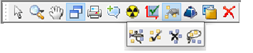
By default, all data points are selected to used by APE, except for the points that are disabled through Data Filter. Additionally, more points can be deselected by using the Tools to Select Data Points for Best Fitting icon from the History plot toolbar:

If it is important to match some specific portion of the data (for example, the first portion of the data, before the end of characteristic flow), you can weight these data points by clicking the Weight Data Points icon ( ). Weighted data points are displayed in a brighter color and are given a 100% weighting.

To specify which parameters to fine-tune, check the automatically calculate variable checkbox to the right of the parameter’s field.

It is important to bound your parameters when you apply the APE, so it gives you values that are meaningful. This can be done by clicking the View Defaults and Limits button to the right of the field.

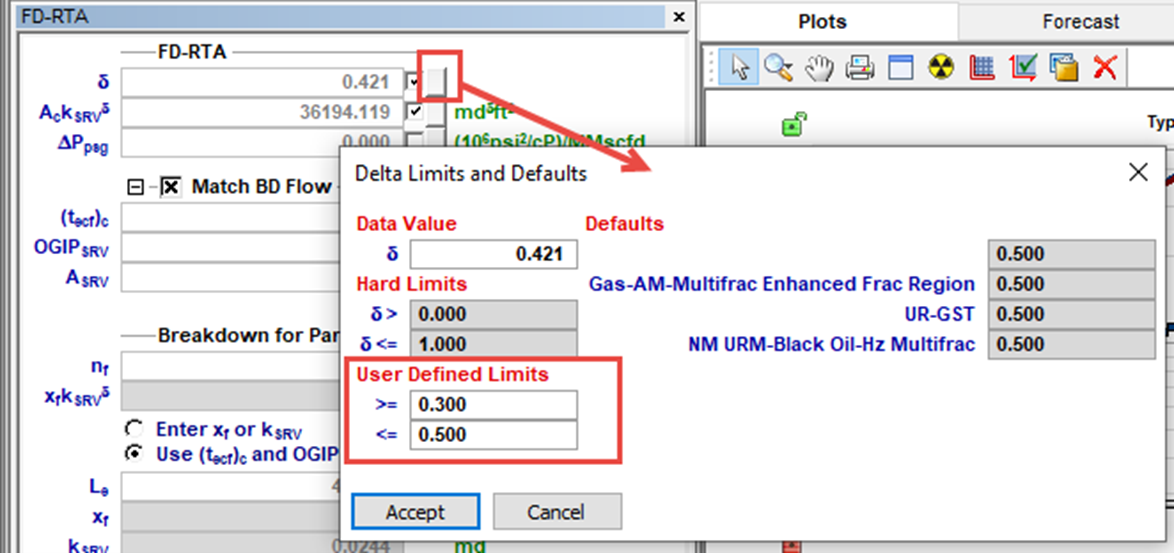
While APE is running, selected parameters are automatically varied to minimize the error between the calculated pressure / rate and the actual pressure / rate depending on the calculation method selected.