Fractional Dimension Rate Transient Analysis Theory (FD-RTA)

Introduction: Classical RTA vs. FD-RTA (for Horizontal Multi-frac wells)

The Classical way to analyse production from Horizontal Multi-frac wells assumes that, fractures are distributed uniformly along the wellbore. In this case, the well experiences linear flow (perpendicular to the fractures) until the transient reaches the boundaries of the SRV.

It has been shown that during the linear flow, the pressure behaviour for a constant rate solution is given by:

Equation 1

For the variable rate case this can be approximated by:

Equation 2

Where t_c is material balance time.

For analysing this type of data, two plots are typically used:

vs. t_c on log-log plot – On this plot portion of the data corresponding to the linear flow follows a straight line with a slope of 0.5.
vs. √(t_c ) on cartesian plot - On this plot portion of the data corresponding to the linear flow follows a straight line with a slope of m

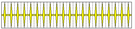
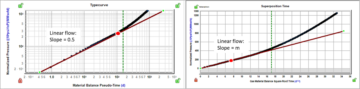
Figure 1

However, actual production from some Horizontal Multi-frac wells does not exhibit this pattern. Instead, early data follows a straight line on the log-log plot, but the slope of this line is not necessarily equal to 0.5. In other words, the flow behavior within the SRV can be described as:

Equation 3

Where δ is a flow dimension parameter (introduced by J Acuna, e.g. URTeC 2118).

This behavior can be attributed to complex fracture networks and non-uniform distribution of fractures along the wellbore. As a result, some of the fractures experience the boundary very soon, while the others remain in linear flow for a longer time. This combination of linear and boundary dominated flow may produce characteristic flow with a slope of (1- δ) on log-log plot. That is, in between linear flow (slope = 0.5) and boundary-dominated flow (slope = 1).

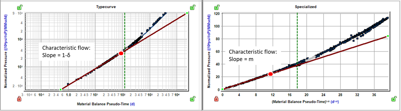
Figure 2

Fractional Dimension Rate Transient Analysis (FD-RTA) is used to analyse, history-match and forecast wells that exhibit such behavior.

Problem definition and analytical solution

With the FD-RTA approach, we do not make assumptions about the actual geometry of the fracture network. Instead, we come up with analogous geometry, that gives the desired pressure response (a solution that follows the desired series of slopes on a log-log plot). The resultant solution can then be used for history matching and forecasting (even though it isn’t based on the actual geometry).

The problem definition and solution below follow Acuña, 2020.

Problem definition

Consider a general case where the desired solution has N slopes (1-δ₁, 1-δ₂, … 1-δ_N) followed by boundary-dominated flow (slope =1).

We start by constructing a proxy model, where all fluid and reservoir properties match those of the actual model. The geometry is depicted as follows:

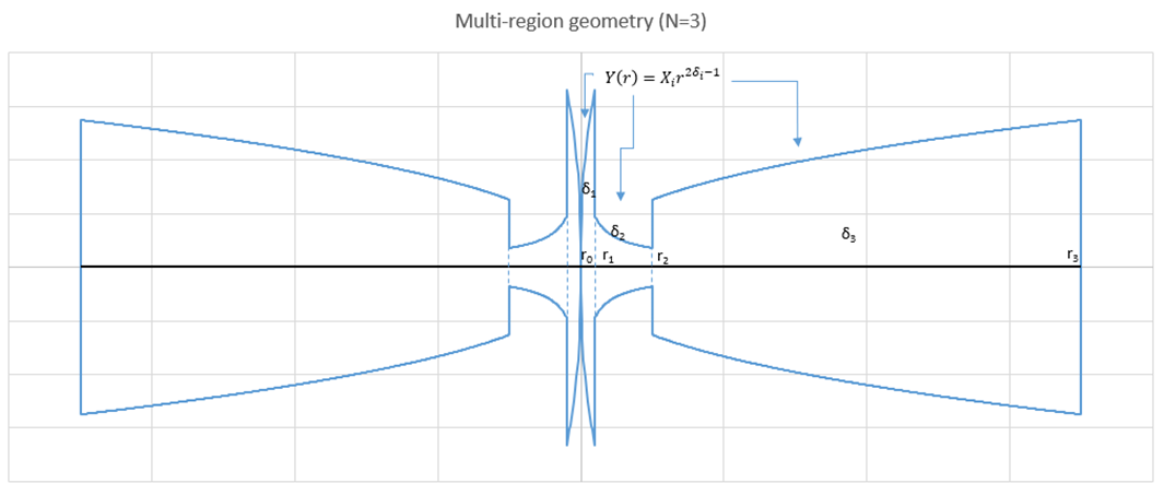
Figure 3

There is just one fracture (and length of the fracture is related to x_ftotal – total fracture half-length of the actual model)
Horizontal direction is denoted as r – distance to the fracture
The whole domain is divided into N regions (in the example illustrated in the figure: N=3)
Each region i spans from r_i-1 to r_i, and for each region, the shape of the boundary is defined as:
Where X₁=x_ftotal, and for other regions X_i is calculated to ensure the continuity of the volume flowing through the r=r_i plane is maintained:
Here r₀ is a small value such that the pressure at r₀ can be interpreted as the wellbore flowing pressure.

One way to understand the way the proxy model is constructed, is to first think of a special case where there is just one region with δ=0.5 (equally distributed fracturs). In this case Y(r)=X₁r^2δ-1=x_ft. Therefore, for this case the geometry of the proxy model reduces to a rectangle that represents fractures stacked on top of each other:

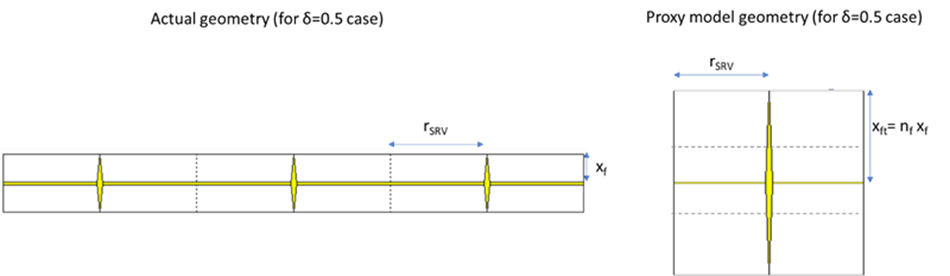
Figure 3a

This special case will result in a solution that follows linear flow (slope = 0.5) followed by boundary-dominated flow.

The intention of building a proxy model for a general case is to get a solution that will follow series of straight-line trends with desired slopes (on log-log plot).

It can be demonstrated (Acuña, 2020) that if we solve the diffusivity equation:

Equation 4

For a system with boundaries defined as shown in Figure 3, the constant rate solution will exhibit the desired slopes on log-log plot.

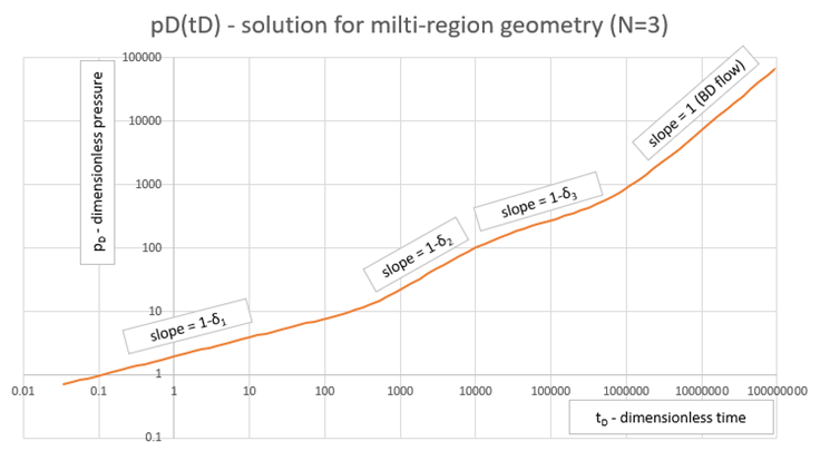
Figure 4

The values of r_i define the duration of each slope. For practical applications, r_i can be used as matching parameters or can be back calculated based on transition times. An example of back-calculation for the SRV-only case is provided later.

Analytical solution

The solution is an adaptation of approach suggested by Abbaszadeh and Kamal (1989). It is defined in dimensionless terms as follows:

Where:

Equation 5

The definitions of p* and t* presented here differ slightly from those used by Acuña (2020) and is consistent with the conventions employed for all analytical modeling calculations in Harmony. Other conversions are adjusted in a way that ensures the resulting solution aligns identically with the one provided in the paper.

Here:

B, bbl/stb – Formation volume factor

µ, cP – Viscosity

c_t, 1/psi – Total compressibility

x_ft, ft – Total fracture half-length (n_fx_f) – used in Equation 10

h, ft – Net pay

_t, fraction – Porosity

k, md - Permeability

p, psi – Pressure

p_i, psi – Initial pressure

t, days – Time

r, ft – Distance from the origin

r_w, ft– Wellbore radius

CF_ph = 141.2 – Conversion factor for pressure

CF_th = 0.0002637*24 – Conversion factor for time

The constant flow rate solution (q=1 stb/day) is calculated in Laplace space as:

Equation 6

Where z is a Laplace space variable, and the remaining functions are defined as follows:

Equation 7

Where I_ᵟ(x) and K_ᵟ(x) are the modified Bessel functions of the first and second kind, respectively.

To calculate θ₁(z) that is used in Equation 6, the following sequence of calculations is used:

Equation 8

Then for i=N-1 to 1:

Equations 9(a-d)

Once is calculated using Equation 6, it can then be converted from Laplace to time domain, to obtain the solution in dimensionless terms, denoted as p_DA=p_DA(t_D).

p_DA(t_D) represents the solution in dimensionless terms used by Acuña (2020). This solution is then adjusted to account for the difference between p* and t* definitions in this formulation as compared to what is used by Acuña (2020).

Equation 10

Once p_D(t_D) is determined, it can be converted into dimensional constant rate solution p_wf=p_wf(t) terms using p*, t* defined in Equation 5.

Equation 11

As mentioned earlier, when we plot the obtained solution on a log-log plot, it follows a sequence of straight lines with slopes of (1-δ_i) – as illustrated in Figure 4.

The conversion from dimensional to dimensionless terms provided above applies to liquids (oil or water). However, the same solution can be applied for gas cases. The only thing that is going to change are definitions of p_D and t_D . For gas, dimensionless pressure is expressed in terms of gas pseudo-pressure, following the same approach as is applied in other analytical model solutions for gas.

Practical application (for SRV-only case)

Directly employing the aforementioned solution requires knowing values for δ, x_ft and k.

If these parameters are known, we can calculate p_wf(t) using Equation 11.

However, in reality values for these parameters are often unknown. The primary objective of the FD-RTA analysis is as follows:

Obtain estimates of the required parameters based on well production data.
Use these parameters to get the constant rate solution p_wf(t).
Generate history match and forecast using this solution.

Let’s begin with considering a simple case involving solely the Stimulated Reservoir Volume (SRV-only case). In this particular case, we make the following assumptions:

The flow from outside the SRV is negligible. (In other words, SRV boundaries are considered to be no-flow.)
The characteristic flow within SRV follows the same behaviour:∆p(t)/q(t)=mt^(1-δ)

Behaviour of constant rate solution for SRV-only case

The geometry of the proxy model for this case has just one segment. Let’s refer to the flow dimension parameter for this segment as δ, and we’ll denote the extent of the segment as r_SRV. In this case the shape of the proxy model looks as on the picture below. (The aim of using the proxy model is to get a constant-rate solution that follows desired sequence of slopes on log-log plot.)

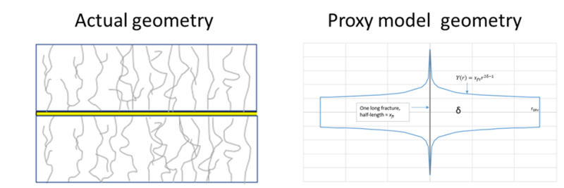
Figure 5

The corresponding constant rate solution (in dimensionless terms) behaves as follows (on the log-log plot):

It follows straight line with a slope of (1-δ) and then transitions to the unit slope (boundary-dominated behavior)
The equation of the straight line (on the log-log plot) during the characteristic flow is:

Equation 12
The time of transition from characteristic flow to boundary dominated (BD) flow can be denoted as (t_ecf)_D where (t_ecf)_D is related to r_SRV by:

Equation 13

The value of c(δ) cannot be precisely calculated; rather it is determined visually based on the point where the solution curve diverges from the first slope. In Harmony, a value of c(δ)=0.5 is employed for consistency with the accepted definition of radius of investigation in linear flow when δ=0.5.

Figure 6

Relation between dimensional and dimensionless Typecurves

The dimensionless typecurve is denoted as p_D(t_D) as defined by Equation 10.

The dimensional typecurve is defined as:

Equation 14

Where p*and t* are defined as per Equation 5.

Note that on log-log plot both p_D(t_D) and (∆p_wf/q)(t) curves exhibit identical shapes, but positions are different. t* moves the curve horizontally and p* moves the curve vertically.

Details of the calculations are given further. But the essence of it is:

We move the dimensionless time curve to pass through the production data
Determine t* and p* by seeing how much the curve moved
Calculate other required parameters using t* and p*.

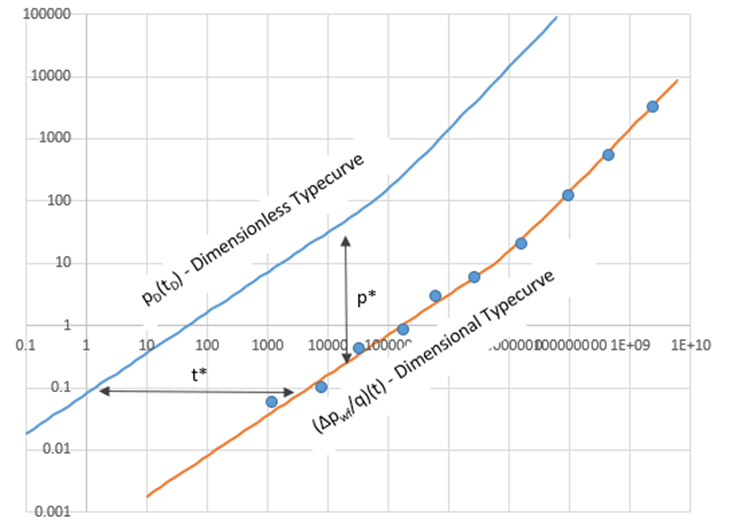
Figure 7

Analysis flow and related calculations

Here is a breakdown of the process for conducting FD-RTA:

The user is presented with an Interactive Typecurve plot: normalized pressure (∆p_wf/q) plotted against (t_c) on log-log plot.
The user identifies the following key elements:

Characteristic flow straight line – This is accomplished by positioning a straight line through the first portion of the data. The equation that represents this line is given as:

Equation 15
End of characteristic flow (t_ecf)_c – The user marks the point where the data starts to deviate from the straight line by placing the vertical line at that position.

Once the values of δ, m and (t_ecf)_c are determined, the subsequent calculations are carried out according to the flowchart below. The equations employed at each step of the diagram are further derived.

Figure 8

Step 1 - Calculate CFP (characteristic flow parameter) based on m:

Equation 16

To derive Equation 16, use:

Equation 17

Next, we convert the equation into dimensionless terms:

Equation 18

Using Equation 10 to replace the left side and multiplying the right side by (r_w^2(1-δ))/(r_w^2(1-δ)):

Equation 19

Then substitute p* and t* using Equation 5 and evaluate at (t_Dr_w²=1). By doing this Equation 19, can be reduced to Equation 16.

Step 2 – Calculate permeability of the proxy model based on t_ecf and r_SRV

We need to come up with a combination of permeability k and size of the proxy model r_SRV, such that the transient response to reach the end of the SRV at the given time t_ecf (since normalized production diverges from characteristic slope at time t_ecf). This combination is non-unique. We can select any arbitrary value for r_SRV (e.g. 1000 ft) and then calculate permeability that would result in the solution that diverges from the straight line at the given time t_ecf:

Equation 20

To derive Equation 20, use Equation 13 and substitute t* from Equation 5.

Step 3 – Calculate total fracture half-length x_ft based on CFP and permeability

Once the permeability k and characteristic flow parameter (CFP=4hx_ft k^δ) are known, the total fracture half-length of the proxy model (x_ft) can be directly calculated.

Step 4 – Calculate area of the SRV (A_SRV) based on x_ft and r_SRV

Considering the geometry as depicted in Figure 5, the area of the model can be calculated by integrating Y(r)=x_ftr^2δ-1:

Equation 21

By using Equation 20 to express r_SRV and subsequently substituting r_SRV in Equation 21, we get:

Equation 22

It is important to note that the calculation in Equation 22 does not involve r_SRV.

Step 5 – Calculate dimensionless Typecurve p_D(t_D) based on δ, r_SRV and x_ft

This can be done by using Equation 10.

Step 6 – Calculate dimensional Typecurve (∆p_wf/q)(t) based on t_D(p_D)

With the permeability of the proxy model determined (Step 2), p* and t* can be calculated using Equation 5. Subsequently the Dimensional Typecurve (∆p_wf(t)/q(t)) can be calculated using Equation 14.

The superposition of this dimensional Typecurve with the historical production of the well gives calculated flowing pressures (p_wf)_calc. This same Typecurve can be used for generating forecasts.

Does this workflow give unique results?

Note that since we initially selected an arbitrary value for r_SRV, the values of k and x_ft calculated using the workflow above, should not be used as estimates for the actual permeability and total fracture half-length of the system. This combination of r_SRV, k and x_ft is just one of the possible combinations that yields the observed pressure response.

However, the resulting dimensional Typecurve (∆p_wf/q)(t) is unique. In other words, if we start with a different value for r_SRV, the corresponding values for k and x_ft will also be different, but the resulting Typecurve (∆p_wf/q)(t) would ultimately be the same.

The value for CFP=A_ck^δ is uniquely calculated based on the combination of δ and m (and does not depend on the choice of r_SRV) as evident from Equation 16.

The value for A_SRV is uniquely determined by the combination of δ, A_ck^δ and t_ecf (and does not depend on the choice of r_SRV) as can be seen from Equation 22.

Breakdown for parameters

As shown above:

The position of the analysis line going though the characteristic flow portion of the data - gives A_ck^δ.
Additionally, you may have the value for A_srv. This value can be acquired from external sources or calculated based on the position of the t_ecf line if the data signature is pronounced enough to be able to uniquely identify the end of characteristic flow.

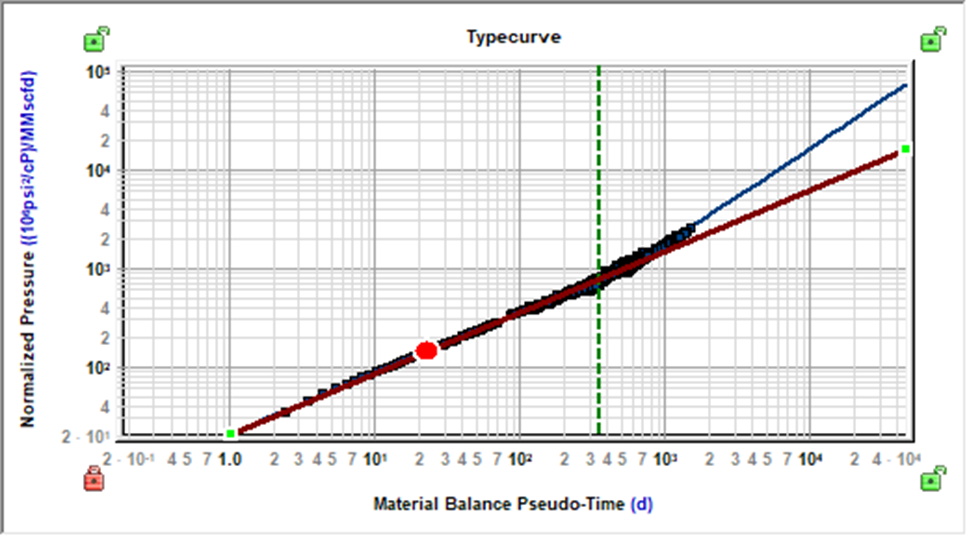
Figure 9

It is important to recognize, that the only direct outputs of the FD-RTA analysis are:

Dimensional Typecurve, which is subsequently used for history matching and forecasting.
Characteristic flow parameter A_ck^δ
A_SRV, provided the production data extends to the end of characteristic flow.

We can further breakdown these parameters assuming that other parameters are known.There are 2 ways this can be done:

Use A_SRV:
- Enter L_e (effective horizontal well length), and x_f will be calculated based on L_e and A_SRV. (A_SRV=2L_ex_f)
- Enter n_f, and k will be calculated based on n_f, x_f and A_ck^δ. (A_ck^δ=4hn_fx_fk^δ)

Do not use A_SRV:
- Enter n_f and one of the k or x_f. The remaining parameter will be calculated based on the one you provide. (Using A_ck^δ=4hn_fx_fk^δ.)

Estimate for permeability

Note that when we calculate permeability k based on x_f and A_ck^δ – the resultant value corresponds to the permeability of the proxy model (as illustrated on Figure 5). However, it is crucial to understand that this permeability is not necessarily equal to the actual permeability of the system and should not be used for reservoir characterization.

Uniquely calculating the actual permeability of the system is a challenging task, because different combinations of fracture distributions and permeability may yield the same response. (One would need additional information about the fracture distribution to do this)

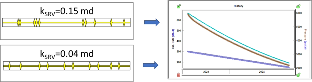
Figure 9a

The case when δ=0.5 (equally distributed fractures) is a special case. In this case, the equation of the boundary Y(r)=x_ftr^2δ-1 reduces to Y(r)=x_ft, resulting in a rectangular boundary. In this case the geometry of the proxy model is equivalent to the actual model geometry and calculated permeability is equal to the actual permeability.

For cases where δ is close to 0.5, the permeability of the proxy model is close to the actual value, so could be used as a rough estimate of the actual permeability. For the cases when δ is far from 0.5, the proxy model’s permeability may be very far from the actual one and should not be used for reservoir characterization.

Accounting for additional pressure drop

Sometimes wells exhibit additional pressure drop, which may be due to damage around the fracture, cleanup, or other reasons. In FD-RTA analyses we model additional pressure drop that is proportional to rate. In this case, the constant rate solution for the system is a modification of Equation 11:

Equation 23

Where ∆P_s (pressure drop due to skin) is a constant.

When the well experiences such additional pressure drop, early data (during flow within the SRV) follows a modification of Equation 3:

Equation 24

This equation can be rearranged as follows:

Equation 25

To analyze data in such cases, it is recommended that users input the value for ∆P_s. Subsequent calculations are then adjusted as follows:

Modification for Typecurve plot:

We plot the adjusted normalized Pressure: (∆p(t)/q(t)-∆P_s) vs. t_c on log-log plot. As per Equation 24, the early data is expected to follow a straight line with a slope of (1-δ) on this plot.

Modification for Specialized plot:

We plot normalized pressure vs. (t_c)^1-δ on this plot. As per Equation 24, the early data is expected to follow a straight line with a slope of m and intersect of ∆P_s on this plot. The interactive line on this plot is moved to account for ∆P_s.

Modification for calculations (history matching and forecast):

The superposition of the modified dimensional Typecurve (as defined in Equation 23) is used for with the historical production of the well gives synthetic calculated flowing pressures (p_wf)_calc. The same modified Typecurve can be used to generate forecasts.

Calculation for related parameters

If the user performs a breakdown for parameters, such that the values for x_f and k_srv are calculated, ∆P_s can be then converted to a more familiar terms of apparent skin (s’) and apparent dimensionless fracture conductivity (FCD’):

Equation 26

Equation 27

Accounting for flow beyond SRV

In the previous section we considered a case where flow from outside SRV was not taken into account. (In other words, SRV boundaries are no-flow).

Now let’s consider a case, where:

The SRV is defined: it has known δ, known CFP and known dimensions. (This means that the flow within SRV follows Equation 24.)
Geometry beyond the SRV is also defined:

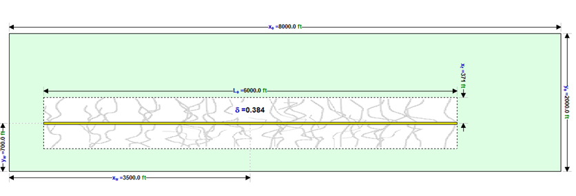
Figure 10

The calculations for such case are a modification of what was proposed by Acuña, 2021 (Urtec 5096).

The calculation can be summarized in the following steps:

Step 1: Calculate r_SRV – half-length of the part of proxy model that represents SRV.
Step 2: Build A(r) function, where r is the distance to the nearest fracture, and A(r) is corresponding area.
Step 3: Divide the entire domain into N regions:
- The first region (0 ≤ r ≤ r_SRV) represents SRV
- Subsequent regions (r_SRV≤ r≤ r₂), (r₂≤ r≤ r₃), … (r_N-1≤ r≤ r_N) represent the area beyond the SRV.
Step 4: Calculate δ_i for each region such that area of each segment is consistent with the A(r) function.
Step 5: Apply correction for δ if necessary.
Step 6: With the proxy model now defined, perfom calculations using this model.

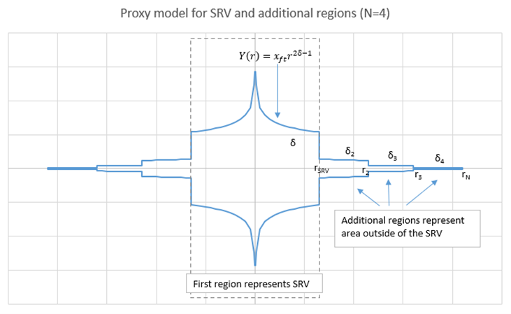
Figure 11

Each of these steps is described in detail below:

Step 1: Calculate r_SRV

Since SRV dimensions are defined, A_SRV can be calculated. A_SRV and r_SRV are then related by Equation 21. We can express r_SRV as:

Equation 28:

The physical meaning of r_SRV is half of the maximum distance between fractures.

For the case with equally distributed fractures (δ=0.5), Equation 28 simplifies to r_SRV=0.5A_SRV/(2_xf)=L_e/(2n_f). In this particular case the geometry of the proxy model is just a rectangle that represents fractures stacked on top of each other:

Figure 12

Step 2: Build A(r) function

Let’s define r as the distance to the nearest fracture. As r increases, the corresponding area A(r) also increases. The area can be calculated as a sum of the part of the SRV that has been investigated and the part of matrix that has been investigated:

Equation 29:

Since the SRV is represented by a segment with flow dimension parameter δ, area of the SRV corresponding to any given r can be calculated by integrating Y(r)=x_ftr^2δ-1:

Equation 30:

The area of the matrix corresponding to any given r can be calculated as illustrated in the image below (the shaded area represents A(r))

Figure 13

Equations 31(a-h):

Step 3: Divide the whole domain into N segments

Use the model geometry to define r_max - the maximum possible distance from the nearest fracture.
Define n=r_max/r_SRV +1.
Choose a value for m, representing the number of external regions to use (Acuña, 2021 suggests using m=5)
Set: r₁=r_SRV, r₂=n^1/m r_SRV , … r_i= n^(i-1)/m r_SRV, …
At this point we have defined the extends of each region.

Step 4: Calculate δ_i for each segment

Now, our objective is to determine δ_i for each region, such that the area of each region is consistent with A(r) function defined earlier.

This approach is taken to build a proxy model wherein the A(r) function mirrors that of the actual model. As a result, we can anticipate that the pressure response of the proxy model will accurately mirror the actual pressure response.

The area of region ‘i’ can be calculated as follows:

Equation 32:

Where X₁=x_ftotal and for other regions, X_i is calculated to ensure the continuity of the volume flowing through r=r_i plane is honored:

It can be shown that Equation 32 is satisfied for each region if we set:

Equation 33:

It is important to note that when r is sufficiently large such that the entire area is covered, the A(r) function becomes constant. When r_i-1 surpasses this value, δ_i becomes 0. At this point we stop adding regions and can use resulting proxy model for calculations.

Step 5: Apply correction for δ (if needed)

Typically, the distance between fractures is considerably smaller than x_f. Consequently, the transient reaches the boundaries of the SRV first, and then the contribution from the matrix becomes significant. A proxy model that has first region representing SRV followed by regions representing matrix is accurate for this case. However, if you set a small n_f, the contribution from beyond the SRV will start making effect before the transient reaches the end of the SRV. In this case:

For the actual model: A(r_SRV) > A_SRV. (By the time the entire SRV is investigated, a substantial portion of the matrix is also explored.)
For the proxy model: A(r_SRV) = A_SRV. (Contributions from the fractures that haven’t reached the SRV boundary are disregarded.)

Figure 13a

This inconsistency might lead to inaccurate results. More than that, there is a possibility that δ_i, as calculated using Equation 33 could surpass 1. This situation would render subsequent calculations impossible.

To avoid this issue we opt to use δ_corrected instead of δ for the first (SRV) region:

δ – is a value provided by user; it describes the characteristic flow (flow within SRV) if there were no contribution from the matrix
δ_corrected- is the value we actually use for the first region. It describes the behaviour of the flow within SRV while considering the presence of some flow from the matrix during the first characteristic flow.
δ_corrected- is iteratively calculated such that the area of the first region of the proxy model equates to A(r_SRV):

Equation 34:

Since δ_corrected is used for the first region, the slope of the typecurve during the characteristic flow period is (1- δ_corrected).

Note that for the cases where contribution from the fracture during the characteristic flow is insignificant, δ_corrected≈δ.

Step 6: Define proxy model and perform calculations

Now that all the necessary parameters for the proxy model have been defined:

First region: use δ_corrected, r_SRV
Subsequent regions: use δ_i as per Equation 33, r_i= n^(i-1)/m r_SRV (as per Step 3)

The diffusivity equation for this model can now be solved as described earlier.

Limitations (for calculation accounting for geometry beyond SRV)

As described above, the method involves building the ‘investigated area’ function A(r). This function describes the investigated area as a distance from the nearest fracture (r). It is important to acknowledge that creating a one-dimensional function A(r) to accurately represent the transient propagation in a two-dimensional system may not always be possible. Therefore, calculations that account for geometry beyond the SRV are approximate.

Below are a few examples where calculation may be inaccurate:

Example 1: Significant contribution from the matrix during the first characteristic flow

When the distance between fractures is high as compared to x_f (Figure 13), part of the matrix will be investigated while the well is still experiencing characteristic flow. In this case it is not possible to accurately describe investigated area as a function of just one variable r. The issue is partially mitigated by incorporating the δ correction; but even with this correction we may end up getting δ_i > 1. In this case further calculation is impossible.

Example 2: directionally incorrect behavior at early time

Consider two cases:

Case 1 – has just the SRV (with certain geometry and δ)
Case 2 – has SRV (with same geometry and δ as for the case 1) with addition of some matrix beyond it.

Both cases are produced at rate control, using same (historical) rate.

Figure 14

The expected behaviour is for Case 2 to exhibit a higher calculated flowing pressure ((p_wf)_calc) due to the additional reservoir volume. In a typical case:

δ_corrected>δ .

The typecurve follows a slope of (1- δ) during characteristic flow, normalized pressure for Case 2 is lower than for Case 1, resulting in (p_wf)_calc for Case 2 being higher than for Case 1 – as expected.

However, it may so happen that during the early time calculation uses the portion of the typecurve below t_D=1. In this case normalized pressure for Case 2 is higher than for Case 1, and the (p_wf)_calc behaves opposite to what is expected.

Example 3: unrealistically large r_SRV

If the value of δ is very small, r_SRV (calculated as per Equation 28) becomes large. In theory it is possible to set up the model in a way that r_SRV>L_e. However, this set up does not reflect any realistic fracture distribution, and the calculation can’t be performed in this case. In this case it is recommended to increase δ. If the data exhibits a steep slope (close to a unit slope), try to match this behaviour by decreasing (t_ecf)_c.

Example 4: high number of regions (N)

As shown in step 3, the sizes of the regions are defined by r_i= n^(i-1)/m r_SRV. Subsequently regions are added incrementally until the entire area is investigated (A(r_N)=A_total). Sometimes this results in a very large number of regions, which makes the calculation unreasonably slow.

This typically occurs when δ>0.5. In such cases, it is recommended to decrease δ. If the data displays a shallow slope, try to replicate this behaviour by using ∆P_s rather than increasing δ.

Modification to model k_matrix < k_SRV

The solution for the diffusivity equation described earlier assumes the same permeability across all regions of the model. However, a modification can be made to account for the cases where k_matrix < k_SRV.

To achieve this, let’s build an analogous model, that has all same parameters as the one we want to use, with just a few exceptions:

Parameter	Original Model	Analog Model	Same or different:
Flow dimension parameter for the SRV:	δ	δ	same
Fracture half-length:	x_f	x_f	same
Well Length:	L_e	L_e	same
SRV permeability:	k_SRV	k_matrix	different
Matrix permeability:	k_matrix	k_matrix	same
Number of fractures:	n_f	n_fcor=n_f(k_SRV/k_matrix)^δ	different
A_SRV:	2L_ex_f	2L_ex_f	same
CFP=A_c(SRV Permeability)^δ:	4hx_fn_f (k_SRV)^δ	4hx_fn_fcor (k_matrix)^δ=4hx_fn_f (k_SRV)^δ	same

As discussed earlier – The k_SRV of the models is not directly used in calculations. The pressure response during the characteristic flow is defined by the combination of the following parameters: δ, CFP and A_SRV. Since both the Original and Analog models share the same δ, CFP and A_SRV values, the pressure response during the characteristic flow period will be identical for both models.

Since both models have same matrix permeability and geometry of the matrix – the pressure response after the characteristic flow is finished, will also be the same between two models. This means, that we could use the Analog model to generate the solution. The Analog model can be calculated as described earlier because it has the same permeability for all regions.