AOF Analysis
Subtopics:
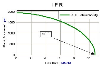
The absolute open flow (AOF) potential of a well is the rate at which the well would produce against zero sandface back pressure. It is used as a measure of gas well performance because it quantifies the ability of a reservoir to deliver gas to the wellbore. Deliverability tests make it possible to predict flow rates against any particular back pressure, including AOF when the back pressure is zero. This result is shown below in an inflow performance relationship (IPR) plot.
| Note: | The AOF and deliverability plots can be generated at both the wellhead and sandface. |
Types of Deliverability Tests
There are a number of tests that can be performed in order to calculate the deliverability of a well as described below.
Conventional Back Pressure Test
The conventional back pressure test is performed by flowing a well at different rates. Each rate is sustained until the radius of investigation has reached the outer edge of the drainage area, and pressure stabilization has been reached. This type of test is not practical for low permeability reservoirs because the time to reach pressure stabilization for each rate is excessive.
Isochronal Test
A fundamental reason that the conventional test is theoretically sound is that the radius of investigation is constant for each flow period. In order to uphold this principle, the isochronal test takes advantage of the fact that the radius of investigation is a function of time and not flow rate.
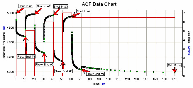
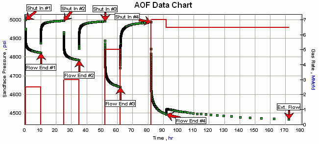
An isochronal test is performed by flowing a well at several different flow rates for periods of equal duration, normally much less than the time required for stabilization. A shut-in, long enough for the pressure to reach essentially static conditions, is performed between each flow period. In addition, an extended flow rate, long enough to reach pressure stabilization, is required.
| Note: | In tight reservoirs, the length of time required to reach pressure stabilization between flow periods could make the isochronal test impractical. |
Modified Isochronal Test
The modified isochronal test is an isochronal test, which requires that each shut-in between flow periods, rather than being long enough to attain essentially static conditions, should be of the same duration as each flow period. It also requires an extended flow period.
Single Point Test
A single point test consists only of an extended flow period, with an estimate of the degree of turbulent flow in the formation. This estimate is often based on information provided by other wells in the same formation, or it can be calculated from reservoir and fluid properties.
AOF Flow Conditions
Extended Flow
Normally an isochronal test includes one flow rate that is extended to stabilization, and a stabilized pressure and flow rate point is determined. This point is the extended flow pressure and flow rate for the test. Single point tests do not include the multi-rate portion of a test and consist of only an extended rate and pressure.
Stabilized Shut-in
Stabilized generally refers to a test in which the pressure no longer changes significantly with time. For AOF tests, the stabilized shut-in pressure is a pressure that reflects the average reservoir pressure at the time. It is either measured during the test, or it is determined from the interpretation of the data.
Stabilized Flow
In high-permeability reservoirs, or wells with small drainage areas, it may be possible to flow the well until stabilization during the extended flow period of a deliverability test. In these cases, the stabilized pressure and flow rate point is the extended flow point.
Many tests however, are not flowed to stabilization because of time constraints (especially in tight reservoirs). An extended flow and stabilized shut-in are still performed at the end of these deliverability tests, so that the buildup data can be analyzed, and from that the stabilized rate calculated. Stabilized flow can be determined by calculation, or by creating a model of the reservoir, doing a forecast at a specified pressure, and finding the point when the rate has stabilized (usually at 3 months, 6 months, or 1 year).
Types of Analyses
Two types of analysis are available: the simplified analysis and the Laminar-Inertial-Turbulent (LIT) analysis.
LIT analysis is more rigorous than the simplified analysis, and is usually only used in tests where turbulence is dominant, and the extrapolation to the AOF is large. However, in most cases the simplified analysis is sufficient to determine the AOF and deliverability.
Pressure Method
For both the simplified and LIT analysis, two pressure options are available, the pressure squared or the pseudo-pressure approach.
Pressure Squared
The pressure-squared approach is the more traditional method, and is often used because it is easier to understand and calculate. However, it is only valid for medium-to-low pressure ranges, but is just as accurate as the pseudo-pressure approach in this range.
Pseudo-Pressure
Using pseudo-pressure is more accurate than the pressure-squared approach, especially when dealing with a high-pressure system, where gas viscosity (mg) and compressibility (cg) cannot be assumed to be constant. Thus, pseudo-pressure works for all pressure ranges, although it is more difficult to calculate and requires more computational time.
Simplified Analysis
The simplified analysis is based on the following equation:
Pressure squared or Pseudo-pressure

The analysis of a modified isochronal test using the simplified method is shown below. For the modified isochronal test, pws must be used instead of pR because the duration of each shut-in period is too short to reach static conditions.
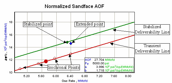
The data is plotted on a log-log plot of Dp2 versus qst where Dp2 is defined as:

The flow and shut-in periods of equal duration provide the information required to plot four points. A straight line, called the transient deliverability line, is drawn through these four points.
The duration of the last flow rate is extended until the pressure response has stabilized. This information is used to plot another point called the stabilized point. A line parallel to the transient deliverability line is drawn through the stabilized point. This is called the stabilized deliverability line.
If the extended flow period does not reach pressure stabilization, a stabilized point can be found by calculation from a buildup test.

The parameter n can be determined from the slope of the line as follows:


Thus, slope is equal to 1 / n, and n is called the inverse slope.
The other parameter, C, can be determined using n and the coordinates (qst and pR) of any point on the stabilized deliverability line (e.g., the stabilized point) as follows:

Note that C and n are considered to be constant for a limited range of flow rates. In theory, it is expected that this form of the deliverability relationship is used only for the range of flow rates used during the test. However, in practice it is used indiscriminately for a wide range of rates and pressures.
LIT Analysis
The Laminar-Inertial-Turbulent (LIT) analysis is used with dealing with high rate wells where turbulence is a major factor. Only the pseudo-pressure approach can be used in this situation since pressures are in a higher range due to the turbulence effects. LIT analysis is defined by the following equation:

Note that the pseudo-pressure squared terms (a qst and b qst2) are equivalent to skin due to damage (sd) and skin due to turbulence (sturb). The coefficients a and b are defined in the example below.
The analysis of an isochronal test using the LIT method is shown below.
Data is plotted on a Cartesian plot of Dy / q versus qst where Dy / q is defined as:

As in the simplified analysis, the transient deliverability line is drawn through the four isochronal points and a parallel stabilized deliverability line is drawn through the stabilized point.
The LIT coefficients, a and b, can be obtained by rearranging the deliverability equation into the form below and plotting Dy / q versus qst on Cartesian coordinates.

From this equation, the slope of the line is equal to b. The parameter a is determined by rearranging the above equation to solve for a and then substituting b and the coordinates (qst and yR) of any point on the line.

References
"Theory and Practice of the Testing of Gas Wells", L. Mattar, G. Brar, and M. Mumby, Energy Resources Conservation Board (1978) Third Edition, Chapter 3.
"Gas Reservoir Engineering", J. Lee and R. Wattenbarger, Society of Petroleum Engineers Inc. (1996) Volume 5, 73 - 74, 173 - 181.