Minifrac After-Closure Analysis
Subtopics:
Soliman / Craig ACA Derivative
Soliman / Craig ACA Bilinear Analysis
Soliman / Craig ACA Linear Analysis
Soliman / Craig ACA Radial Analysis
After-closure analysis is performed on the portion of the falloff data collected after the induced fracture closes. Unlike traditional pressure transient analysis (PTA), which is founded on the “constant-rate solution”, the main after-closure analysis (ACA) techniques are founded on the “impulse solution”. The fundamental difference is that the “constant-rate solution” hinges on the flow rate prior to the analyzed shut-in period, whereas, the “impulse solution” hinges on a “defined volume”. Impulse solutions are used because of the short injection period and assume that the entire injected volume is injected instantaneously. In practice, the injection of fluid occurs over a period of time. Therefore, the data does not follow the characteristic derivative response until the falloff duration is much larger than the injection period. However, there are different implementations of the “impulse solution” that can lead to different interpretations.
In WellTest, the after-closure analysis is divided into these categories:
- After-closure Diagnostic (Nolte) based on the work of K.G. Nolte.
- After-closure Diagnostic (Soliman / Craig) based on the work of M.Y. Soliman and the work of D. Craig.
It is possible to obtain reasonable estimates of reservoir pressure and formation permeability from diagnostic analyses if the pressure falloff is recorded long enough to achieve radial flow. Minifrac analytical models provide the significant advantage of verifying and improving on results obtained from diagnostic analyses, similar to the analysis workflow used for many years in traditional PTA. With modeling, you can match transitions between flow regimes and you do not need to depend on the identification of fully developed flow regimes.
Nolte
This after-closure analysis method is based on the work of K.G. Nolte, and expanded on by R.D. Barree. It is based on the solution of a constant pressure injection followed by a falloff. The impulse equations are obtained by approximating the injection duration as very small. Nolte's techniques use injected volume as the impulse volume and consider the closure point as the beginning of the falloff.
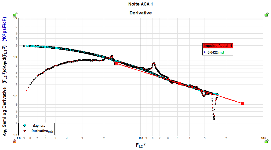
Nolte ACA Derivative
The Derivative plot is used to identify flow regimes. Impulse Linear and Radial flow have slopes of -1/2 and -1, respectively, when their semi-log derivative is plotted on the log-log Derivative plot.
After net pay, porosity, and fluid saturations have been entered, analysis lines may be added. The initial reservoir pressure defaults to the p* (extrapolated pressure) of the first analysis line added. This default may be overridden manually by typing a value into the initial pressure cell of the Parameters dialog box, or a default value from another analysis line can be used by clicking the Default button beside the initial pressure cell. If the initial pressure is linked to an analysis line, it updates as the line is moved. The delta pressure curve on the Derivative plot is defined as the measured falloff pressure minus the initial pressure.
If impulse radial flow is identified, the pressure data overlays the derivative data. This diagnostic may be used to help fine-tune the estimate of initial pressure.
Nolte ACA Linear Analysis
If impulse linear flow is identified, the fluid loss coefficients, CR and CT, can be estimated.
The equation governing impulse linear flow is defined as:

There are two MiniFrac ACA (Nolte) Linear Time functions. FL1 is an approximation of FL2. The above equation holds regardless of the linear time function used.
Impulse linear flow shows up as a straight line on a plot of pressure vs. FL (FL1 or FL2).
An impulse linear analysis line can be added from the Analysis Options dialog box. The impulse linear line should then be positioned through the linear flow portion of the falloff data (identified by a straight line on the MiniFrac Linear plot, or a -1/2 slope on the Derivative plot). When the impulse linear line is selected, the Analysis Options dialog box displays cells for entering closure pressure and permeability, as shown below. The closure pressure is obtained from the pre-closure analysis. If radial flow developed, permeability could be estimated from the Impulse Radial analysis. Otherwise, a best estimate of permeability must be entered in order to estimate the fluid loss coefficients.
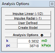
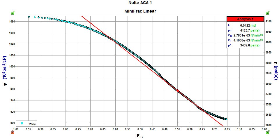
After closure pressure and permeability have been specified, the position of the impulse linear line is used to calculate p* and fluid loss coefficients, CR and CT. Both MiniFrac ACA (Nolte) Linear Time functions are bounded by 1.0 (at early shut-in time) signifying the time of closure and 0.0 (at late time) representing an infinite shut-in time. P* is the extrapolation of the linear line to FL= 0, which corresponds to an infinite shut-in time.
Fluid Loss Coefficients:


CT is the total fluid-loss coefficient.
CR is the reservoir fluid-loss coefficient.
p@tc is the extrapolation of the
linear flow line at closure time, tc.
Note: FL = 1.0 at tc
pi is the estimated initial pressure.
Nolte ACA Radial Analysis
If impulse radial flow is identified, the extrapolated pressure, p*, and permeability can be estimated.
The MiniFrac Nolte ACA Radial Time function, FR1, has a minimum value of 0.0 (at late time) representing an infinite shut-in time. p* is therefore obtained from the extrapolation of the linear line to FR1= 0. As described in Reference 1 (Barree, 2007), the equation governing impulse radial flow is defined as:

The radial flow portion of the after-closure falloff data has a straight-line trend on a plot of pressure vs. FR1.
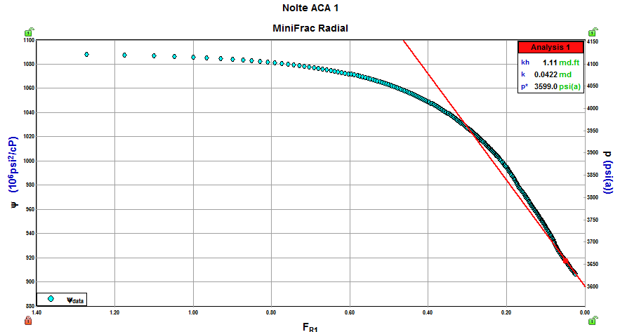
An impulse radial analysis line can be added from the Analysis Options dialog. The impulse radial line should then be positioned through the radial flow portion of the falloff data (identified by a straight line on the MiniFrac Radial plot or a -1 slope on the Derivative plot).
The slope of the line on the MiniFrac Radial plot is mR1 and permeability may be calculated as follows:


With the position of the impulse radial line on the Derivative plot, you can form a similar calculation:


Soliman / Craig
M.Y. Soliman's solutions for short-term tests are also useful in the analysis of Minifrac tests. These solutions have been implemented in WellTestTM. In his derivation, Soliman assumed a constant rate injection and falloff sequence. He applied superposition in Laplace space to obtain a single equation and then took the late-time approximation to obtain impulse equations (for bilinear, linear, and radial flow). Because his late-time approximations are designed for short injection and long falloff periods, Minifrac tests can be analyzed using his solutions.
D. Craig developed an analytical model that accounts for fracture growth, leakoff, closure, and after-closure. The late-time approximation of his model produced impulse radial and bilinear flow equations that are the same as Soliman's solutions. However, the constant in Craig's impulse linear flow equation differs from Soliman's. The linear flow equation implemented in the Soliman / Craig analysis method in WellTestTM uses the constant obtained by D.Craig.
| Note: | Soliman / Craig's solutions facilitate the use of analytical models. |
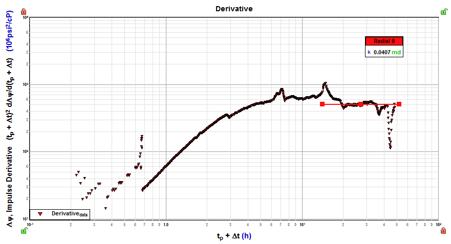
Soliman / Craig ACA Derivative
The Derivative plot is used to identify flow regimes. Impulse Bilinear, Linear, and Radial flow have slopes of 1/4, 1/2, and 0, respectively, when their impulse derivative is plotted on the log-log Derivative plot. The impulse derivative is used, instead of the semi-log derivative, to produce diagnostic plots in which the flow regimes have characteristic slopes identical to those noted in conventional well test interpretation.
After net pay, porosity, and fluid saturations have been entered, typecurve lines may be added.
By default, the delta pressure curve is not displayed on this plot. It can be added by right-clicking the legend and selecting to view the delta pressure curve from the customization menu. The delta pressure curve on the Derivative plot is defined as the measured falloff pressure minus the initial pressure. The initial reservoir pressure defaults to the p* (extrapolated pressure) of the first late-time analysis line added. This default may be overridden manually by typing a value into the Initial Pressure field of the Parameters dialog box, or by using the default value from another analysis line by clicking the Default button beside the Initial Pressure field in the Parameters dialog box. If the initial pressure is linked to an analysis line, and if delta pressure is displayed on the typecurve, the delta pressure updates as the line is moved.
Soliman / Craig ACA Bilinear Analysis
If bilinear flow is identified, the fracture conductivity, kfw, can be estimated.
The equation governing bilinear flow is defined as:

Therefore,
bilinear flow shows up as a straight line on a plot of pressure vs. 
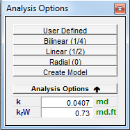
A bilinear analysis line can be added from the Analysis Options dialog box. The bilinear line should then be positioned through the bilinear flow portion of the falloff data (identified by a straight line on the MiniFrac bilinear plot, or a 1/4 slope on the Derivative plot). When the bilinear line is selected, the Analysis Options dialog box displays a field for entering permeability, as shown below. If radial flow developed, permeability could be estimated from the Radial analysis. Otherwise, a best estimate of permeability must be entered. After permeability is entered, fracture conductivity is calculated.
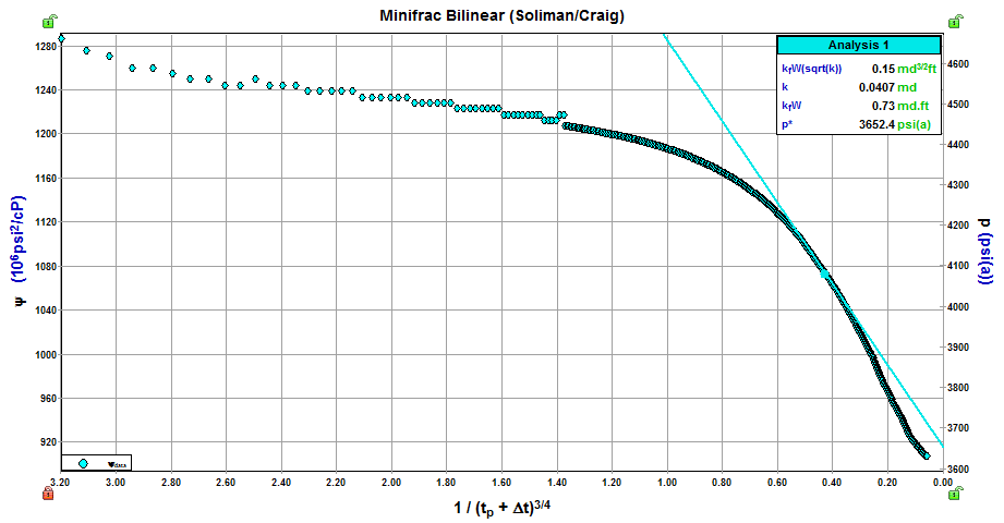
As shown in the equations below, the slope of the bilinear line yields kfw * sqrt(k). Permeability must be estimated in order to calculate fracture conductivity.


Soliman / Craig ACA Linear Analysis
If linear flow is identified, the fracture half length, Xf, can be estimated.
The equation governing linear flow is defined as:

Therefore,
linear flow shows up as a straight line on a plot of pressure vs.

A linear analysis line can be added from the Analysis Options dialog box. The linear line should then be positioned through the linear flow portion of the falloff data (identified by a straight line on the MiniFrac linear plot, or a 1/2 slope on the Derivative plot). When the linear line is selected, the Analysis Options dialog box displays a field for entering permeability, as shown below. If radial flow developed, permeability could be estimated from the Impulse Radial analysis. Otherwise, a best estimate of permeability must be entered. After permeability is entered, fracture half-length is calculated.
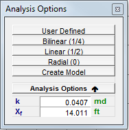
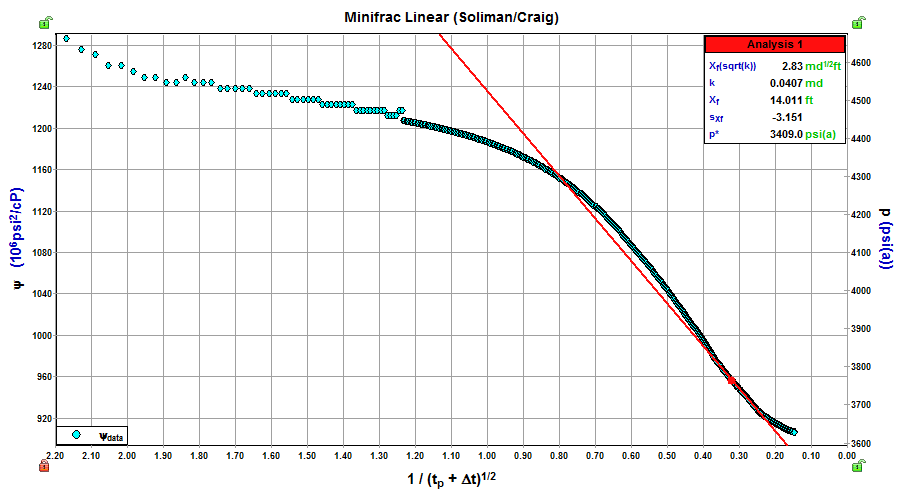
As shown in the equations below, the slope of the linear line yields Xf * sqrt(k). Permeability must be estimated in order to calculate fracture half-length.


Soliman / Craig ACA Radial Analysis
If radial flow is identified, the extrapolated pressure, p*, and permeability, k, can be estimated.
The equation governing radial flow is defined as:

The MiniFrac Soliman / Craig ACA Radial Time function has a minimum value of 0.0 (at late time) representing an infinite shut-in time. p* is the extrapolation of the radial line to the time of 0, which corresponds to an infinite shut-in time.
The
radial flow portion of the after-closure falloff data has a straight-line
trend on a plot of pressure vs.

A radial analysis line can be added from the Analysis Options dialog box. The radial line should then be positioned through the radial flow portion of the falloff data (identified by a straight line on the MiniFrac radial plot, or a zero slope on the Derivative plot).
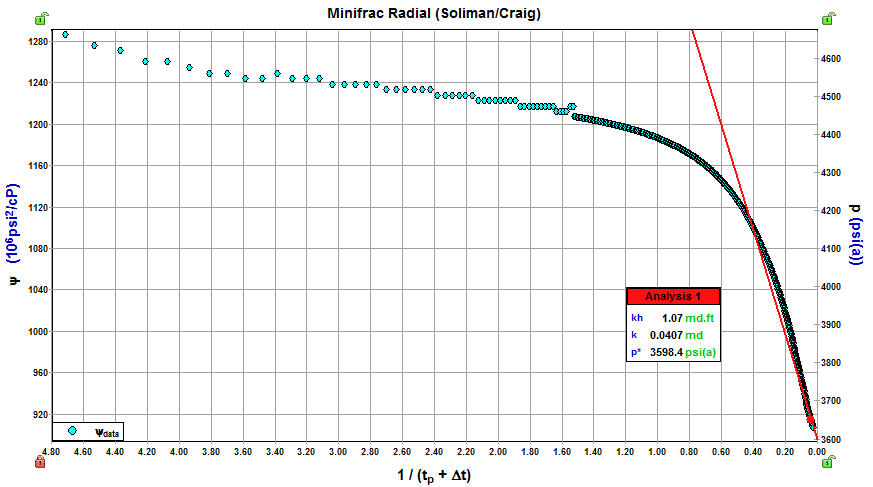
As shown in the equations below, permeability can be estimated from the slope of the line on the radial plot.


