Performing a Minifrac Analysis

Performing a Pre-Closure Analysis

To perform a pre-closure analysis (PCA):

1. Click the Analysis menu and select Pre-closure Diagnostic.

A new tab opens (e.g., PCA Diagnostic 1).

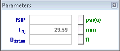
2. Enter Datum Depth (TVD) in the Parameters dialog box. This is used to calculate the ISIP (Instantaneous Shut-In Pressure) gradient, which is displayed on the parameter annotations on the pre-closure analysis plots after ISIP has been identified.

3. Identify ISIP.

4. Identify closure.

Performing a Nolte After-Closure Analysis

To perform a Nolte after-closure analysis (ACA):

1. Click the Analysis menu and select After-closure Diagnostic (Nolte).

A new tab opens (e.g., Nolte ACA 1).

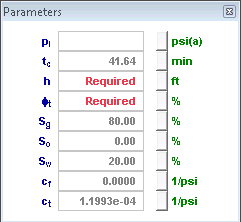
2. Enter net pay (h) and porosity (phi) in the Parameters dialog box.

3. Identify flow regimes. On the Derivative plot (i.e., bottom-left plot), look at the slope of the semi-log derivative data. A well established slope of -1 indicates radial flow has developed, and a slope of -1/2 indicates linear flow.

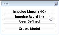
4. Add analysis lines.

If radial flow was identified, click the Impulse Radial button in the Lines dialog box.

If linear flow was identified, click the Impulse Linear button in the Lines dialog box.

5. Position the lines through the appropriate after-closure data. Click and drag the center point of the line on the Derivative plot. On the specialized plots (Minifrac Radial or Minifrac Linear plots), you may also click and drag the center point of the line, or click the line to rotate it.

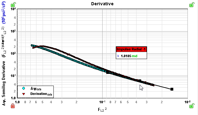
Radial flow gives an estimate of p* and permeability. Linear flow yields leakoff coefficients.

Note:

If radial flow was not identified, place a radial flow line at the end of the after-closure data to get upper limits of permeability and p*.

Performing a Soliman / Craig After-Closure Analysis

To perform a Soliman / Craig ACA:

1. Click the Analysis menu and select After-closure Diagnostic (Soliman/Craig).

A new tab opens (e.g., Soliman / Craig ACA 1).

2. Ensure net pay (h) and porosity (phi) have been specified in the Parameters dialog box.

3. Identify flow regimes. On the Derivative plot (i.e., bottom-left plot), look at the slope of the semi-log derivative data. A well established zero slope (horizontal trend) indicates radial flow has developed, and a slope of +1/2 indicates linear flow.

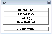
4. Add analysis lines.

If radial flow was identified, click the Radial button in the Lines dialog box.

If linear flow was identified, click the Linear button in the Lines dialog box.

5. Position the lines through the appropriate after-closure data. click and drag the center point of the line on the Derivative plot. On the specialized plots (Minifrac Radial or Minifrac Linear plots), you may also click and drag the center point of the line, or click the line to rotate it.

Radial flow gives an estimate of p* and permeability. Linear flow yields X_f*sqrt(k).

Note:

If radial flow was not identified, place a radial flow line at the end of the after-closure data to get upper limits of permeability and p*.

History Matching Minifrac After-Closure Data

To history match minifrac after-closure data:

1. Create a legacy model:

If radial flow was identified, select Vertical from the Model menu.
If linear flow was identified, select Fracture with Boundaries from the Model menu.

A new tab opens (e.g., Vertical 1).

2. Enter required parameters:

Vertical Model: enter a skin of -3 to initialize the model.
Fracture with Boundaries model: initialize Xf and k if estimates were not obtained from the Soliman After-Closure Analysis.

3. History match the after-closure data.

Note:

A good match is not possible based on pre-closure falloff data.