Performing a PITA Analysis
To perform a performance inflow test analysis (PITA) analysis:
1. If the PITA test was performed on a vertical well, click the Analysis menu and select Vertical Diagnostic. Or, if it was performed on a horizontal well, click the Analysis menu and select Horizontal Diagnostic. ![]()
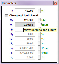
2. Enter pay (h) and porosity (Φ) in the Parameters dialog box. Enter effective horizontal well length (Le) for a Horizontal Diagnostic. ![]()
Note: The pay thickness (h) for a PITA test in a vertical well is usually entered as the height of the perforated interval.
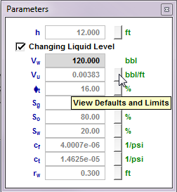
3. Decide whether there is a changing liquid level in the wellbore. If there is a changing liquid level, it dominates the changes in pressure in the wellbore, and you should click the Changing Liquid Level checkbox within the Parameters dialog box. If a single-phase exists in the wellbore, changes to pressure in the wellbore are controlled by compressibility.
Note: The Changing Liquid Level option is not available for PITA inflow tests in gas reservoirs.
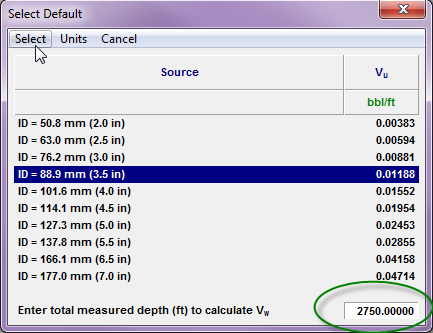
4. If the Changing Liquid Level checkbox is not selected (e.g., for a PITA inflow test in a gas reservoir):
- Click the button beside the Vw field.
- Select the casing size from the list of common casing IDs (inner diameters). Enter the measured depth of the well and click Select. A calculated value is displayed in the Vw field in the Parameters dialog box.
The Select Default dialog box opens.
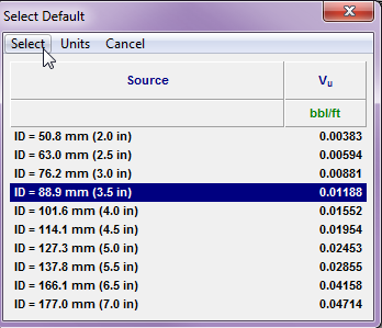
5. If the Changing Liquid Level checkbox is selected:
- Click the button beside the Vu field.
- Select the casing size from the list of common casing IDs and click Select. A calculated value is displayed in the Vu field in the Parameters dialog box.
The Select Default dialog box opens.
6. Identify flow regimes. On the Derivative plot (i.e., bottom-right plot), look at the slope of the semi-log derivative data. A well established zero slope (horizontal trend) indicates radial flow has developed, a slope of 1/2 indicates linear flow, and a slope of 1/4 indicates bilinear flow.
7. Add analysis lines. ![]()
- If radial flow was identified, click the Late Time-Impulse Radial button in the Lines dialog box.
- After an impulse radial line has been added, the Early Time +ve and -ve Skin buttons are enabled. If you do not know if the skin is positive or negative, you can add both and see which skin value makes the most sense.
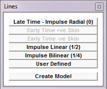
If radial flow was not identified, you may wish to place a radial flow line at the end of the data to get estimates of permeability and p* to initialize the reservoir model.
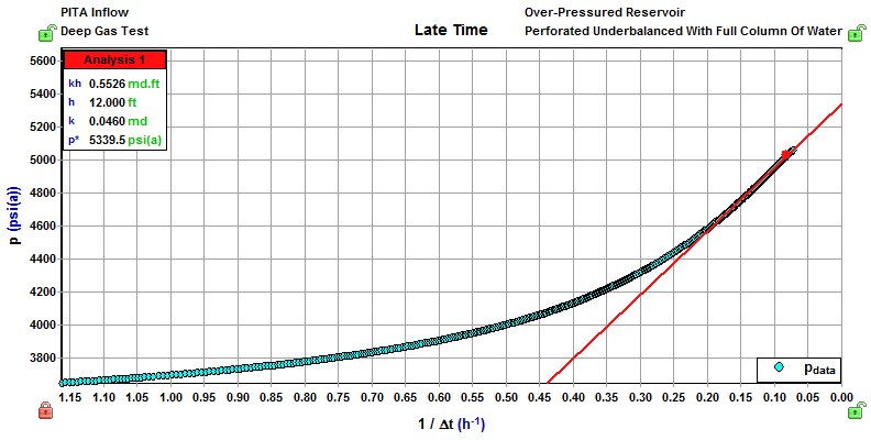
8. Position the lines through the appropriate data. Click and drag the center point of the line on the Derivative plot. On the specialized plots (e.g., Late Time), you may also click and drag the center point of the line, or click the line to rotate it.
Note: The impulse radial line yields estimates of permeability and p*. The early time lines yield estimates of skin.
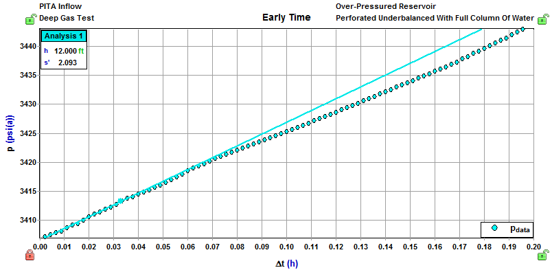
9. Select the Early Time +ve Skin line from the Analysis Lines box.
This line is displayed on the Early Time plot, and you can use it to estimate skin.
| Note: | The bottom-left plot (history plot) contains a line representing the calculated inflow or injection rate. This is additional information, which is not required for any part of the analysis. |
History Matching PITA Data
To history match PITA data:
1. Click the Model menu and select a model. In most PITA tests performed on vertical wells, a vertical model is used for PITA tests.
A new tab opens (e.g., Vertical 1).
2. History match the PITA data. Focus on the late-time data to try to get estimates of permeability and pi.
You may decide to do a history match to get more accurate results. For additional information, see History Matching Overview. For a PITA test, we recommend doing the history match on the Late Time plot.