Hybrid Model Theory
Subtopics:
General Formulation for the Single-phase Model
Well Constraint Considerations
Considerations when Estimating Fluid Properties
Hybrid Model Pseudo-pressure Definition
Hybrid Model Pseudo-pressure Formulation
Advantages of Using the Pseudo-pressure Formulation
Background
There are two main types of models used to simulate the flow of fluid through porous media: analytical models and numerical models. Both types have their advantages and disadvantages.
Analytical Models
Analytical models have relatively short calculation times, so you can history match with these models quickly. More than that, you can even match the model automatically using APE.
The main disadvantage for these models is that they can only simulate single-phase flow – either liquid or gas, but not gas and liquid flowing together. Additionally, analytical models do not fully account for changing fluid properties with pressure. In case of liquid flow, fluid properties are assumed to be constant, and in case of gas flow, the change of fluid properties with pressure is accounted for by using pseudo-pressure and pseudo-time.
Unfortunately, pseudo-time is not an exact transformation. As a result, changing gas properties are only accounted for to a certain extent. Therefore, in cases where pressure varies significantly across the reservoir (e.g., pays with low permeability), long-term forecasts for gas analytical models may be inaccurate. There is no known way to fully account for the change in fluid properties when using analytical models.
Numerical Models
With numerical models, you can model multiphase flow, and account for changing properties of each phase, and the interaction between phases.
The main disadvantage for these models is their long computation time. With the numerical model,the reservoir is divided into a number of cells, and then the flow is modeled simultaneously in all cells. To be able to assume constant pressure and constant fluid properties within each cell, the size of each cell needs to be relatively small. Therefore, the number of cells required for an accurate solution becomes large, which results in a long computation time. Note that decreasing the number of cells to reduce computation time may significantly affect calculation results.
Performing a manual history match for numerical models is time consuming. In addition, an automatic history match for numerical models is complicated, and thus not widely available in commercial software.
Hybrid Model
The hybrid model is essentially a numerical model, but with certain modifications to significantly reduce computation time, so that it is almost as fast as an analytical model. These modifications include:
- accounting for one phase only (gas)
- using the pseudo-pressure formulation
General Formulation for the Single-phase Model
To calculate pressure across the reservoir, we divide it into a number of grid cells. At each timestep (n+1), we formulate a material balance for each cell.
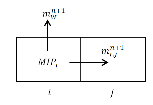
To define components of mass balance for cell i at timestep n+1:
Mass in place (MIP) for cell i at timestep n+1 can be calculated as:
Equation 1

where:
Vbi = bulk volume for cell i
pin+1 = pressure for cell i at timestep n+1
φ = porosity
ρ = density
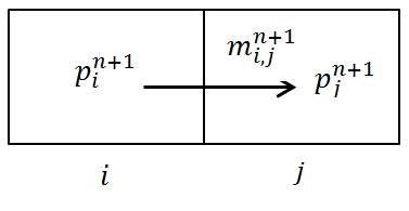
Mass flow from cell i to the adjacent cell j during timestep n+1 can be calculated as:

(We used Darcy’s Law to calculate flow rate.)
In equation 2:
 = flow rate from cell i to cell j at timestep n+1
Ai,j = cross-section area between cells i and j
Li,j = distance between the centers of cells i and j
μ = viscosity
k = permeability at the initial pressure
km(p) = permeability multiplier (permeability at a certain pressure is calculated as  ).
).
Mass produced at the well during timestep n+1 (if well penetrates cell i) can be calculated as:

where:
WI = wellbore index (as per Peaceman 1978 or Babu and Oden, 1989)
 = pressure at the wellbore at timestep n+1
Material balance for cell i at timestep n can be written as:
Equation 4

Using equations 1, 2, and 3, and bringing all the terms to the left, we can rewrite equation 4 as:

Assuming that the pressure distribution has been calculated for timesteps 1, 2, ... n, to calculate pressure distribution at timestep n+1, we formulate material balance (equation 5) for each cell, and solve all these equations simultaneously. Unknowns of the system are  for each cell i; therefore, the number of equations is the same as the number of unknowns, and the system can be solved.
Well Constraint Considerations
For a well producing at a specified sandface pressure, the described system of equations can be used directly (because  is known). However, for a well that produces at a specified surface q, an extra equation is required.

where:
i = summation index for all cells penetrated by the well
ρsc = fluid density at standard conditions
Considerations when Estimating Fluid Properties
In the above formulation, we use rock and fluid properties estimated at certain pressures. The term  is used in
  (equation 2) and in
  (equation 3).
Some logical questions are:
- At what pressure should we estimate this term?
- Should we use pressure in one of the cells, or some kind of average?
If the modeled fluid is liquid, its properties do not change much with pressure; therefore, pressure in any cell can be used.
In the case of gas flow, properties significantly vary with pressure; therefore, selecting the correct way of estimating properties becomes important.
In classical numerical simulation (including numerical models in Harmony), properties are estimated at the pressure of the upstream cell (i.e., the cell with the higher pressure). For such a simulation to be accurate, you should ensure that properties in the adjacent cells are close. This could be achieved by having small grid cells. Unfortunately, having smaller grid cells results in longer computation times.
With the hybrid model, we use the pseudo-pressure formulation to estimate fluid properties.
Hybrid Model Pseudo-pressure Definition
Hybrid model pseudo-pressure is defined as:

| Note: | The definition of hybrid model pseudo-pressure is very similar to a traditional pseudo-pressure. To see this, express density as  (z = gas compressibility factor, T = temperature, R = gas constant, M = molar mass). This results in the following equation: (z = gas compressibility factor, T = temperature, R = gas constant, M = molar mass). This results in the following equation: |
Equation 8

Therefore, the hybrid model pseudo-pressure and traditional pseudo-pressure are different by a constant factor.
Hybrid Model Pseudo-pressure Formulation
As was mentioned in Considerations when Estimating Fluid Properties, the calculation of mass flow from one cell to another given in equation 2 has a deficiency: it does not account for a variation of fluid properties with pressure. The hybrid model formulation modifies equation 2 to get a relationship between the mass flow rate and pressure drop when properties are changing with pressure.
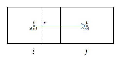
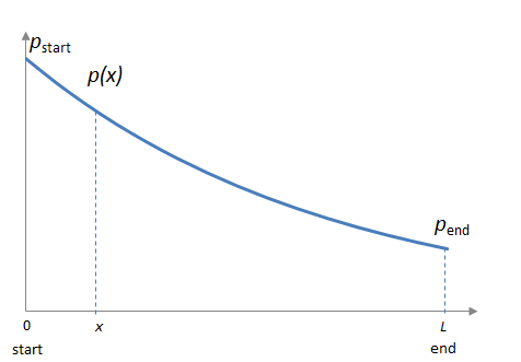
At each cross-section at any given distance (x), the pressure gradient across the cross-section can be expressed using the differential form of Darcy’s Law:
Equation 9

where  is the mass flow rate across the cross-section. This can be re-arranged as:
Equation 10

Integrating both parts from 0 to L with respect to x, and using the left-side of the equation is a constant with respect to x, we get the following equation:
Equation 11

| Note: | We used the definition given in equation 7 for the last transformation. |
To summarize, when fluid properties are changing with pressure, the mass flow rate through the cross-section can be calculated as:
Equation 12

Therefore, equation 2 can be modified to account for changing properties. The mass flow from cell i to cell j during timestep n+1 is calculated as:
Equation 13

Equation 3 can be modified in a similar fashion. Mass produced at the well during timestep n+1 is calculated as:

As a result, the material balance equation for each cell (equation 5) is modified to:

Assuming that the pressure distribution has been calculated for timesteps 1, 2, ... n, to calculate pressure distribution at timestep n+1, we formulate a modified material balance (equation 14) for each cell, and solve all these equations simultaneously. Unknowns of the system are  for each cell i; therefore, the number of equations is the same as the number of unknowns, and the system can be solved.
| Note: | Well constraints are treated in a similar way to general numerical model formulations. |
Advantages of Using the Pseudo-pressure Formulation
Pseudo-pressure formulation makes simulation significantly faster than classical numerical simulation modeling for the following three reasons:
1. Smaller number of grid cells: In classical numerical simulation, grid cells have to be small enough to consider constant fluid properties within each cell. Pseudo-pressure formulation accounts for a variation of fluid properties between the centers of two adjacent cells; therefore, it is possible to have larger grid cells. By having a smaller number of grid cells, calculation speed increases.
2. Faster solution for a non-linear system: While performing numerical modeling, equation 5 is solved at each timestep. This system of equations is non-linear; therefore, it is solved iteratively, using the Newton-Raphson method. This method involves calculating derivatives of each matrix element with respect to each unknown. Calculating these derivatives is faster for pseudo-pressure formulation (equation 14), because we have to deal with one fluid property function ( ) as opposed to a combination of three functions (
 ) for traditional formulation. More than that, due to the integral nature of
  , its derivative is calculated easily.
3. Symmetry: When it comes to solving systems of equations, there are faster algorithms available for the case when the matrix of the system is symmetrical. Therefore, another advantage of using the formulation given in equation 14 over equation 5, is that equation 14 forms a symmetrical matrix, while estimating properties at the upstream cell for equation 5 results in an asymmetrical matrix.