Numerical Model Theory

Subtopics:

Differences between Black Oil, Gas Condensate, and Volatile Oil Models

Black Oil and Modified Black Oil Properties

Numerical Modeling Using Modified Black Oil Properties

Considerations when Using Numerical Simulation

Numerical models offer a more detailed method of modeling pressure / rate data by dividing the reservoir into smaller blocks. Rigorous material balance calculations are performed on each block to account for diffusion based on permeability, saturation, porosity, and fluid properties. Variations in these parameters can be rigorously accounted for which gives the numerical models a huge advantage over conventional analytical models, which assume a homogenous reservoir with constant reservoir and fluid properties. Numerical models are ideal for modeling multiphase situations where you may have solution gas in addition to changing saturations.

The underlying assumption of the analytical models for production data analysis is single phase flow in the reservoir. In order to accommodate multiple flowing phases, the model must be able to handle changing fluid saturations and relative permeabilities. Since these phenomena are highly non-linear, analytical solutions are very difficult to obtain and use. Thus, numerical models are generally used to provide solutions for the multiphase flow problem. (The numerical engine used in the software is based on a general purpose black-oil simulator.) Numerical models can be created with less simplifying assumptions for reservoir properties than analytical models. The reservoir heterogeneity, mass transfer between phases, and the flow mechanisms can be incorporated rigorously.

Numerical models solve the nonlinear partial-differential equations (PDEs) describing fluid flow through porous media with numerical methods. Numerical methods are the process of discretizing the PDEs into algebraic equations, and solving those algebraic equations to obtain the solutions. These solutions that represent the reservoir behaviour are the values of pressure and phase saturation at discrete points in the reservoir and at discrete times.

The advantages of the numerical method approach are that the reservoir heterogeneity, mass transfer between phases, and forces / mechanisms responsible for flow can be adequately taken into consideration. For instance, multiphase flow, capillary and gravity forces, spatial variations of rock properties, fluid properties, and relative permeability characteristics can be represented accurately in a numerical model. In general, analytical methods provide exact solutions to simplified problems, while numerical methods yield approximate solutions to the exact problems. One consequence of this is that the level of detail and time required to define a numerical model is more than its equivalent analytical model.

Differences between Black Oil, Gas Condensate, and Volatile Oil Models

To account for differences between black oil, gas condensate, and volatile oil models, we need to introduce various properties.

Black Oil and Modified Black Oil Properties

With the modified black oil PVT model, reservoir engineers can account for complex PVT behaviour that arises in gas condensate and volatile oil reservoirs.

Gas-condensate and volatile oil systems contain gas that may have non-negligible amounts of vaporized liquid hydrocarbons, and this may have a significant impact on fluid behaviour.

Common black oil numerical formulations do not consider changes in the liquid hydrocarbon content of the gas phase. In the modified black oil model, two new properties are added to account for the liquid contained in gas:

1. vaporized oil ratio (R_v).

2. dry gas formation volume factor (B_gd).

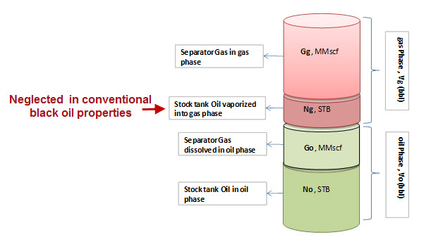
To explain these new properties, consider the figure below, which illustrates the distribution between the phases at given reservoir conditions. Excluding water, in both black oil and modified black oil modeling, it is assumed that there are two components (separator gas (G) and stock tank oil (N)), and two phases (gas phase (g) and oil phase (o)); and each of these components can exist in either phase. The amount of the produced gas at the separator is the summation of gas components that come from the gas phase (G_g), and the gas component that comes from the oil phase (dissolved gas, G_o). Likewise, the stock tank oil (N) comes from both the oil phase (N_o) and the gas phase (vaporized oil, N_g):

N_g is neglected in the conventional black oil numerical formulation, but is honoured in the modified black oil numerical formulation.

The Vaporized oil ratio (R_v) for the gas phase is defined an being analogous to the solution gas ratio (R_s) for the oil phase. Physically, if a gas sample at reservoir conditions is brought to standard conditions, R_v describes the volume of hydrocarbon that condensates into liquid, per volume of separator gas produced (typically expressed as bbl/MMscf). For a specific liquid-rich gas system, the vaporized oil ratio (R_v) is a function of pressure, temperature, and separator conditions, and the Ovalle correlation for R_vis available.

Dry gas formation volume factor (B_gd) is another distinct modified black oil property. The wet gas formation volume factor (B_g) is defined as the ratio of the gas phase volume at a given pressure and temperature (V_g) to the equivalent volume of the whole gas phase at standard conditions:

The dry gas formation volume factor (B_gd) is the ratio between the volume of the gas phase at given conditions (V_g) to the volume of its gas component (G_g) at standard conditions:

In conventional black oil applications, N_g is zero, which causes B_gdand B_gto become the same. However, for modified black oil applications, we need to differentiate between B_gand B_gd. Although there is no correlation available for B_gd, it can be calculated by using the following relationship between B_gand B_gd (Whitson and Brule, 2000):

where:

• α - conversion factor (1 bbl = 5.615 ft³)
• ρ_oST - oil density at standard conditions (stock tank)
• M_oST - stock tank oil molecular weight
• R - universal gas constant
• T_SC - standard condition temperature
• P_SC - standard condition pressure

Numerical Modeling Using Modified Black Oil Properties

All the original (black oil) numerical models in WellTest 2013 v2 (v 7.7.0) and older, use black oil properties. Therefore, the simulation results for gas condensates and volatile oil reservoirs may not be fully accurate in some cases. Particularly for gas condensate reservoirs, the original numerical models cannot predict the condensate drop-out in the reservoir, which affects both condensate surface yield and well productivity.

The Gas Condensate and Volatile Oil Numerical models use modified black oil properties; therefore the condensate drop-out is modeled correctly.

Gas Condensate Numerical models use the Gas Rate and Condensate Rate columns from the Production Editor tab as an input for production data. Condensate properties are set in the Properties tab’s Oil section. The Gas Condensate Numerical model reports dry gas rates and condensate rates.

Volatile Oil Numerical models use the Gas Rate and Oil Rate columns from the Production Editor tab as an input for production data. The Volatile Oil Numerical model reports dry gas rates and oil rates.

Before a Gas Condensate Numerical model or Volatile Oil Numerical model starts a simulation, WellTest verifies that the properties entered into the simulators are physically meaningful. The model performs multiple property consistency checks, and if these checks do not meet the established criteria, an error or warning message is displayed. The checking criteria are as follows:

p_bp = p_dew

Other checking criteria:

At any pressure:

c_o > 0

c_g > 0

At any pressure where p ≤ p_bp or p_dew:

ρ_o ≥ ρ_g

1 / R_v ≥ R_s

B_gd / R_v ≥ B_o

B_o / R_s ≥ B_gd

μ_o ≥ μ_g

At p = p_bp or p_dew:

c_o (at p = p_bp) ≥ c_o (at p > p_bp)

c_g (at p = p_dew) ≥ c_g ( at p > p_dew)

Considerations When Using Numerical Simulation

Speed: Numerical models are more computationally intensive and slower than analytical models.

Simulation can stop: Although the numerical engine is robust, there are several cases that cause the execution of the model to fail. (This is true of any gridded simulator.) This usually happens when the model shortens its time steps too much, such as when there are rapid operational changes in rate or pressure. These issues can usually be overcome by smoothing the data, and eliminating dramatic shifts in rate and/or pressure.

Numerical Errors: There are several types of errors associated with the numerical solution. The first type is called truncation error, which is caused by a truncated Taylor series expansion replacing the spatial derivative and time derivative. The order of truncation error is proportional to Dx (grid size) and Dt (time-step size). This implies that as Dx and Dt decrease, the truncation error decreases. However, both decreased grid size and time-step size result in an increased number of computational operations, which introduces additional error called computational round-off error. Therefore, the tradeoff between truncation error and round-off error should be examined carefully.

There is another kind of approximation that can result in one more type of error that is caused by the well model incorporated in the numerical model.  In order to obtain the accurate wellbore pressure or flow rate, very fine grids around the wellbore are required. This is especially critical for compressible fluids and low permeability reservoirs. The best gridding method around the well is cylindrical grids, but they are only applicable for single-well modeling.

Gridding: Fine gridding is required to obtain the pressure or flow rate at the wellbore. This is especially true for compressible fluids and low permeability reservoirs.  Although cylindrical grids provide the best solution around the wellbore, they can't be used for multi-well modeling. Cartesian gridding is the most common grid type used in the industry. The Peaceman Wellbore Index model for Cartesian grids is used by most general numerical simulators, but can overestimate the wellbore pressure, if rate is the constraint, and overestimate rate, if pressure is the constraint. It also produces artificial wellbore storage (afterflow) effects during the early transient period. Our numerical models use the Peaceman Wellbore Index model for vertical wells, and the Babu and Odeh Wellbore Index model for horizontal wells.