Using the Numerical Model

After the numerical model is set up, it is available for your use.

Note:   Before the model starts a simulation, it performs multiple consistency checks on the input properties.

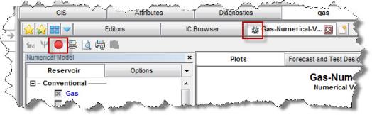
1. Run calculations by clicking the Synthesize icon () on the toolbar.

While the model is calculating, you will see a rotating gear on the header of the tab. To stop the simulation, click the Stop Simulation () icon.

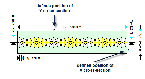
While the model is calculating, you can see how the spatial distribution on pressure changes with time. Both top and cross-section views are available. The position of the cross-section is defined by the blue triangular sliders on the schematic plot.

2. You can replace one or more plots on the dashboard by clicking the Add an available view icons.

3. Once the calculation is finished, you can see how pressures or saturations change through time by clicking the playback icons (highlighted in the screenshot below) on any Color Shading plot.

4. To display grid lines on the top view, click the Toggle Grid Lines icon ().

5. To display the legend, click the Toggle Color Legend icon ().

6. To history match the model, change the parameters manually. Most of the history matching parameters are located on the History Model pane. However, you may also want to change some parameters located in the Properties Editor (e.g., relative permeability curves, R_s curve, R_v curve, etc.).

Once the model has been populated and calibrated to the production and pressure data, production forecasts can be created and compared under a variety of different constraints. The procedure for forecasting using a numerical model is similar to Forecasting Using Analytical Models.

Note:   Wellhead forecasting is not currently available for the numerical models.