Tight Gas / Shale Decline Analysis Theory

Tight Gas Reservoirs

A tight gas reservoir generally refers to a reservoir of natural gas with an average permeability of less than 0.1 mD. The structure of a tight reservoir is typically a gas-bearing sandstone or carbonate matrix (may contain natural fractures). Often the pores are poorly connected by very narrow capillaries resulting in very low in-situ permeability. Gas flow rates through these rocks are generally low and often more complex well completions are necessary to achieve economic levels of production.

Shale Gas Reservoirs

The gas storage mechanism in a shale gas reservoir is unlike that of a conventional gas reservoir. In a typical gas reservoir, gas is stored in the pores by compression. In  coalbed methane (CBM, coal seam gas) or shale reservoirs, gas is stored within the coal/shale matrix by adsorption, in addition to the free gas stored in the fracture network. For more information, see Langmuir Isotherm - Adsorption. As the reservoir pressure is reduced, gas is desorbed from the surface of the matrix. It then flows into the fracture network, allowing for the production of the gas.

Tight Gas / Shale Decline Analysis

In tight gas/shale production, the duration of transient flow is much longer than conventional production. Traditional decline methods assume boundary dominated flow, and are not correctly used during transient production data. Many authors have investigated modifying traditional decline curve analysis to forecast production from tight gas reservoirs. Unfortunately, most methods are complicated and dependent on pressure data that may not be available to the user.

When decline analysis has been used in tight gas/shale gas production, a harmonic or superbolic decline (b value of 1 or greater) results. Specifically, linear flow can be demonstrated as a decline exponent of 2. In these cases, there are instances where the effective decline rate becomes very low (approaching zero) and the expected ultimate recovery (EUR) interpreted is an overestimate. Before the development of the tight gas/shale Decline method, the limiting effective decline rate (dlim) approach had been used to impose a dlim value. The effect of dlim is to replace the hyperbolic decline with exponential once it reaches the specified decline rate. Often this minimum decline rate is arbitrarily chosen.

In the tight gas/shale Decline method, when boundary-dominated time (tBDF) is reached the decline exponent (b) can be decreased from the transient match to a reasonable value for boundary dominated flow (b ≤ 0.5).

Comparison of Decline Methods

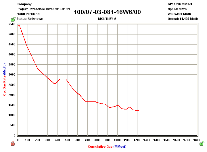
In the well shown, only a small portion of transient production is available. There is a large range of recoverable volumes that may result when trying to create a forecast based on this data.

Figure 1: Three Months of Production in Montney Shale

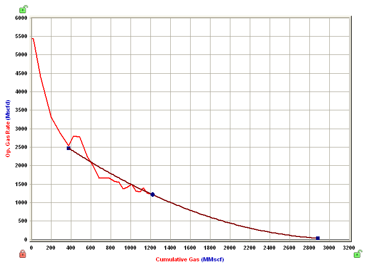
A conservative approach would be to fit a hyperbolic trend to this data. The results will significantly underestimate the production of this well.

Figure 2: Hyperbolic Decline, b = 0.5

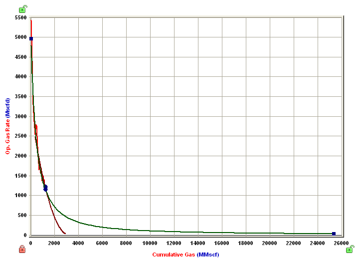
Typical shale production shows a rapid decline in early production followed by very flat stable rates for an extended period. Before shale production was better understood, many analysts used superbolic decline exponents for the entire forecast period. The figure below compares this to the hyperbolic decline. It is clear that superbolic decline is an overestimate of the recoverable gas.

Figure 3: Comparison of b = 0.5 and b = 1.7

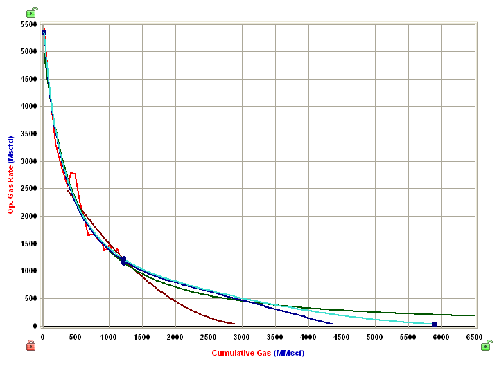
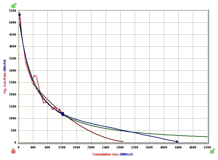
With the modified hyperbolic, dlim, you can use a larger decline exponent while limiting how low the decline rate becomes. In this case, hyperbolic decline with a limited effective decline rate of 10% is used. It provides a more optimistic forecast than hyperbolic decline, but restricts the unreasonably low decline rates shown in superbolic decline forecasts. However, in practice the dlim is often selected arbitrarily.

Figure 4: Comparison of Hyperbolic, Superbolic, and dlim Decline

Finally, with the tight gas decline approach, you can incorporate geological information into the interpretation. In this case, the permeability is approximately 0.01 mD and the wells are drilled on 80 acre spacing. By entering these parameters, the tBDF is calculated to be 50 months. The defaults of bTRAN = 2.0 and bBDF = 0.5 are used. This creates a forecast similar to dlim, but the later decline exponent can be greater than 0, which is not commonly observed in gas production. The end result is a reasonable forecast with parameters selected appropriate to the production scenario.

Figure 5: Comparison of Hyperbolic and Tight Gas Decline