You are here:

Data diagnostics theory

The analysis of production data to determine reservoir characteristics, completion effectiveness, and hydrocarbons-in-place is becoming more prevalent. The methods of analysis have been documented and verified in numerous publications. The concepts underlying modern production data analysis are the same as pressure transient analysis. Even though both these domains use the same underlying theory of fluid flow through porous media and can determine the same variables (permeability, skin, reservoir size), it should not be assumed that they can replace each other. Pressure transient analysis and production data analysis must be viewed as complementary and not substitutes for each other. Pressure transient analysis deals mostly with “high frequency / high resolution” shut-in data, while production data analysis deals with “low frequency / low resolution” flowing data. This in itself, presents significant differences in data quality and interpretations.

Like all mathematical solutions, production data analysis methods are subject to numerous assumptions, which often can be justified. In this case, if the data is complete, consistent and of good quality, meaningful results can be obtained. However, if the quality of the data is questionable, then the production data analysis methods should be used with caution. In this case, the analyst’s ability to filter out the bad data and extract the true reservoir signal becomes extremely important. As mentioned by Anderson et al. 2006, blind application of production data analysis methods without consideration of data quality issues can lead to misinterpretation of the reservoir characteristics. An analyst, who is not experienced in recognizing such inconsistencies, can obtain an answer that appears to be mathematically correct, yet be completely wrong because of using “bad data” for analysis.

There is no complete set of criteria that covers all of the challenges and pitfalls in production data analysis. Some inconsistencies in data measurement or reporting are more critical than others, while the same issue may be critical in one situation, but not in another. This makes data diagnostics complicated and very dependent on the expertise of the analyst. Nonetheless, there are some issues that are worse than others, and cause “bad” or inconsistent production data a lot of the time. Some of the more common issues are listed below:

Missing flowing pressures — Even though the rate history is carefully obtained from daily records, the pressure history is infrequent, inaccurate, or often non-existent.
Missing flow rates — Even though the flowing pressure of an individual well is obtained accurately and frequently from permanently installed downhole gauges, the corresponding flow rate is often non-existent, or has been pro-rated on a monthly basis from a group meter of several wells.
Rate or pressure averaging — Often the flow rate and/or the flowing pressure are measured at high frequency (every minute), but for data storage efficiency, are averaged to daily quantities. Depending on the rate variations during that period, this may result in meaningless numbers.
Wrong initial pressure — The initial pressure is unknown or wrong, especially in tight gas or infill drilling.
Liquid loading — The calculation of sandface pressures is wrong due to the unknown “standing liquid column” in the wellbore.
Wrong pressure source and flow path — If the source of the wellhead pressure measurement or the flow path are specified incorrectly (tubing, annulus or both, or changing from one to the other) the calculated sandface pressures will be incorrect.
Wrong production data — Rate allocations to individual wells based on group metering can be in error, as the distribution is based on infrequent tests.
Wrong production data — The water production rate of individual wells is often poorly monitored or misreported. While small quantities of water may have little effect on the reservoir interpretation, they can have a significant effect on the wellbore performance and on the calculation of sandface pressures from wellhead data.
Significant increase in water / gas ratio — When the water-gas ratio is high (>100 bbl/MMscf), the assumption of single-phase Darcy flow in the reservoir may not be valid, or the skin due to water coning may be variable, which affects the validity of the permeability and skin calculations.
Operational modifications:

Opening up of new perforations / shutting off old perforations
Refracturing of the well
Changing tubulars
Changing flow path

Wrong location of pressure gauge — Often the only flowing pressure available is the pressure downstream of the choke. If the choke is wide open, this pressure is usable, but if the choke is being used to control the flow rate, then the downstream pressure is not of much value.
Wrong rate and pressure synchronization — The original rate and pressure data often have different time tracks, and if they have not been synchronized properly, the interpretation may be invalid.

Sometimes a simple look at the reported production data (flowing pressure, gas and liquid flow rates and time) can reveal obvious or potential inconsistencies, or provide insight for interpretation. Here are some examples:

If the flow rate suddenly increases, the flowing pressure should abruptly decrease correspondingly.
If the flow rate is below the “critical liquid lift velocity” calculated using Turner correlation (Turner et al. 1969) or Coleman correlation (Coleman et al., 1991), there is the likelihood of liquid loading.
If the tubing and casing pressure profiles are diverging, it is an indication of liquid load-up.
The pressure is measured every minute but reported daily, along with the daily average rate. If there have been interruptions or significant rate changes during the 24-hour interval, an average daily rate is meaningful, but an average daily pressure is not.
Sometimes the flow rate is pro-rated from a group-meter measurement instead of being measured at the individual well. The pro-rating formula honors the total production from all the wells, but may be completely incorrect at the individual well level, especially when there have been undocumented production disruptions at various wells.
A rapid increase in the water-gas ratio could indicate water coning, and wellbore operational problems.
A rapid decrease in the water-gas ratio or condensate-gas ratio could indicate liquid loading in the wellbore.
A high frequency of scatter in production rates, pressures, the water-gas ratio, or condensate-gas ratio can indicate unstable flow in the well and/or unstable operating conditions.
Flat (constant) liquid production rates, with large step changes, usually indicate infrequent measurement. The presence of this kind of data can make the quality of the calculated sandface pressures low, even if the wellhead pressures are of high quality.
No liquid rates are reported, yet either the pressure data indicates “slugging”, or it is a known fact that liquids are being produced. In this case, the quality of the calculated sandface flowing pressure may not be high, even if the wellhead pressures are of high quality.
Flat (constant) pressures with step changes usually indicate infrequent pressure measurement. This means that one pressure is recorded per week or month, and then it is reported as a constant value until another reading is taken.
Straight-line trends in pressures or rates usually indicate infrequent measurements and interpolation between them (rather than actual measurement).

Note:

For additional data diagnostic examples, see the data diagnostics flowchart.

When an analysis is performed, the analyst must always review the interpretation to make sure it makes sense. This is the ultimate test and must never be avoided. Although it is preferable to identify and eliminate inconsistent data before the analysis is undertaken, sometimes inconsistencies do not become evident until after the analysis has been completed. For example, a sudden change in the slope of the flowing material balance plot (p/Z plot) is a diagnostic that depends on information about original-gas-in-place, which is obtained from interpretation.

Recognizing the fact that the analysis and interpretation of production data is influenced significantly by the quality and consistency of the data, it is the objective of this topic to develop a series of diagnostic plots and guidelines that can help analysts to identify “bad data” and prevent misleading answers resulting from analyzing poor-quality data. The diagnostic plots are independent of any interpretations as they are considered pre-analysis diagnostics.

To achieve the objective of this topic, a number of diagnostic plots are proposed. These plots are then used in a number of case studies using field examples. The intent was to investigate if these diagnostics plots could differentiate between “good data” and “bad data”. The results of this study allow production engineers to recognize poor-quality data, and avoid being misled by their results, or at least to make a reasonable judgments as to the quality of their interpretations.

Production data diagnostics

There are four areas of investigation in production data diagnostics:

1. Outlier removal

2. Liquid loading in the wellbore

3. Single phase flow in the reservoir

4. Consistency (correlation) between rate and pressure

Outlier removal

The first step in production data diagnostics is the removal of outliers. Apart from adding extraneous noise to what is often an already confusing mass of data, these outliers can cause incorrect interpretation if they are not removed. For example, often outliers show a unit slope on typecurves. This unit slope may be easily misdiagnosed as reservoir depletion. It should not be used as an indication of original-gas-in-place or of boundary-dominated flow. A simple solution is to simply identify and remove the outliers from the analysis.

Liquid loading in the wellbore

In this step, the analyst should investigate if there is any issue with liquids loading up in the well, or if there is any unstable flow in the well. If liquid loading exists, and the sandface flowing pressure is being calculated from wellhead measurements, it is very easy to get the wrong answer, because multiphase flow calculations do not account for “stagnant” liquid columns in the wellbore. The following points should be considered in this step:

If the pressure data is measured at the mid-point of perforations (MPP), then liquid loading or any other wellbore issues will not affect production data analysis. However, any correction from the gauge depth to the MPP can be a source of error (sometimes significant, depending on the distance between them).
If the sandface pressure is being calculated from wellhead measurements, and the “quiet side” is being used (for example, the well is flowing through tubing and the pressure source is the annulus), the calculation down to end-of-tubing (EOT) is often very good. However, from the EOT to the MPP, there often exists a “stagnant” liquid column, which must be accounted for by estimating a “flowing” gradient (estimated at 0.2 - 0.3 psi/ft or 4-7 kPa/m for water).
If the sandface pressure is being calculated from wellhead measurements, and the “flowing side” is being used, multiphase flow calculations must be used, and their accuracy (unless calibrated to similar flowing conditions) is questionable.

The following plots can be used to identify liquid loading. (Some of the plots can be used to identify productivity issues as well as liquid loading.)

Gas rate and sandface pressure versus time — If there is a high degree of scatter in production rates and pressures, then it indicates unstable flow in the well, like slugging, and/or unstable operating conditions.
Difference between casing and tubing pressure versus time — The tubing and casing pressure profiles should track each other if there is no problem in the wellbore. The plot shows that if the difference between casing pressure and tubing pressure is changing (diverging tubing and casing pressures with time), then there is possibility of liquid loading.
Water-gas-ratio or condensate-gas-ratio versus time — A fluctuation or rapid decrease in the water-gas ratio and condensate-gas ratio is an indication of unstable flow in the well. Fluctuation is an indication of slug flow and a rapid decrease is an indication of liquid loading. If slug flow is indicated, yet no water rate is reported, then the quality of calculated sandface pressures may be questionable, even if the wellhead pressures are of high quality.

The water-gas ratio versus time plot has another practical importance. A rapid increase in the water-gas ratio could indicate possible productivity issues related to water (for example, water coning), as gas relative permeability decreases significantly at high water-gas ratios.

log (q) versus log (t) — This plot has diagnostic value in cases where the gas rate is decreasing abnormally as a result of liquid loading or any other productivity issues. The log scale tends to compress the late-time data and accentuate the declining rate trend in the late-time data. This plot may also accentuate the fluctuation in gas rate, which can be useful to identify slug flow.

All the above indicators of wellbore liquid problems must be viewed together, as they are often complementary effects, but some of them may be more evident than others.

Single-phase flow in the reservoir

A plot of the water-gas ratio versus time is used in this step. If the water-gas ratio is high, the assumption of single-phase flow in the reservoir may not be acceptable. A threshold value for the water-gas ratio should be defined (suggested value of 100 bbl / MMscf), and the portion of the data with a water-gas ratio higher than the threshold value should not be used for analysis using typecurves and analytical models, as these analysis methods are developed assuming single-phase flow inside the reservoir.

Consistency (correlation) between rate and pressure

After removing the outliers, and the data which indicates liquid loading and productivity issues in the wellbore, and/or multiphase flow inside the reservoir, the analyst should look for consistency between pressure and rate data. If the rate and pressure data are inconsistent with each other, they should be identified and should not be used to interpret reservoir effects (permeability, skin or gas-in-place). The series of Diagnostic Plots described in the following section are recommended for use in identifying or accentuating any such inconsistency.

The concept of a diagnostic plot implies that a certain feature or behavior emerges from a given data profile. More specifically, diagnostic plots should highlight that the data is “bad” by indicating that a certain expected feature does not exist, or that the displayed profile deviates significantly from expectations. When this occurs, the apparent signal is potentially misleading and the wrong reservoir interpretation would be extracted, if the analyst proceeds. As explained by Anderson et al. 2006, a diagnostic plot for production data should:

Highlight that there is something wrong with the production data.
Identify the causes of misbehavior, if any exist.
Show if the flow rate and flowing pressure are correlated or not.

The diagnostic plots for identifying inconsistent production data are described below:

Gas rate and sandface pressure versus time — Visually check for a negative correlation between rate and pressure data. This means that if the flow rate suddenly increases (or decreases), then the flowing pressure should decrease (or increase) correspondingly. If that does not happen, the rate and pressure data are inconsistent with each other, which may be because the rate is wrong, or the pressure is wrong, or the completion has changed (for example, refrac, tubing change).
If the rate changes by an order of magnitude, it is better to use log (q) instead of q.
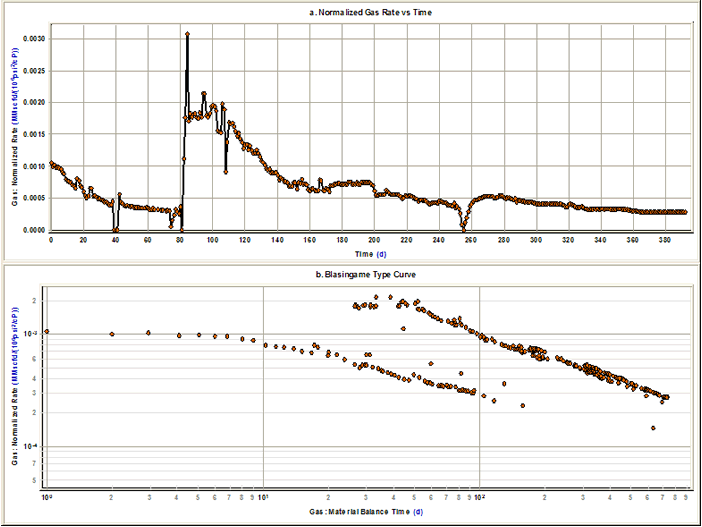
Normalized rate versus time — This is a plot of q / Δpp versus time. In the absence of step changes in rate and pressure, theory indicates that q / Δpp must decrease continuously with time. Therefore, an increasing trend in q / Δppwith time indicates that non-reservoir effects are present. Note that if there are different stems in the q / Δpp versus time plot and q / Δpp is decreasing with time in each stem, (see Figure 1a), the analyst should not conclude that the rate and pressure data are inconsistent, as these different stems can be caused by step changes in rate and/or pressure. However, it forces the analyst to ask the question: Is there any inconsistency between rate and pressure data?
Normalized pressure versus time—This is a plot of Δpp / q versus time. The trend of the plot is the reverse of the q / Δpp versus time plot. However, the signature and diagnostic value tends to be the same. In general, whenever a plot of q / Δpp is used, pretty much the same information could have been obtained by plotting Δpp / q instead. The choice of one or the other is a personal preference.
Percentage drawdown versus time — This plot shows [ (Δp / pi) *100 ] versus time, and indicates the degree of drawdown. Knowing the degree of drawdown can be an important issue in production data diagnostics because theory indicates that the pressure variable to be used for analysis should be Dp (= pi - pwf). If Dp / pi is close to unity, then we are dealing with a well with high drawdown, and in this case, the effect of pi overshadows that of pwf, and makes the rate insensitive to variations in the flowing pressure. In other words, any discrepancies in flowing pressure will not have much of an effect on rate. For example, if there is a step change in flowing pressure, this step change may not be reflected in the rate (given normal data scatter). In the case of high drawdown, even if the flow rate and pressure are not correlated, the diagnostic plots which depend on Dp may not indicate that there is a problem.
The fact that high drawdown yields pressure-insensitive rates is a diagnostic onto itself. This is very useful when public data is analyzed, as often, all or part of the pressure data is missing from the production file. If we know that the well is producing under high drawdown conditions, then the rate is insensitive to flowing pressure and any discrepancies in flowing pressure do not really matter.
Blasingame typecurve — This is a log-log plot of normalized rate (q / Dpp) versus material balance time, (that is, Gp / q), where Gp is the cumulative production of gas and q is the gas rate. Theoretically, normalized rate must decrease continuously with material balance time. Therefore, an increasing trend indicates that non-reservoir effects are present. If there are step pressure or rate changes, they will cause a sudden deviation from the decreasing trend, but the general trend will be resumed if the data is consistent. However, if there are different stems in this plot, it is an indication of inconsistency between rate and pressure data (see Figure 1b).
NPI typecurve — This is a log-log plot of normalized pressure (Dpp / q) versus material balance time (Gp / q). This plot is the inverse of the Blasingame plot. Theoretically, the normalized pressure must increase continuously with material balance time. Therefore, a decreasing trend indicates that non-reservoir effects are present. If there are different stems in this plot, it is an indication of inconsistency between rate and pressure data.
FMB rate — This is based on the flowing material b Balance (FMB) concept. It is a Cartesian plot of normalized rate (q / Dpp) versus normalized cumulative (Gp / Dpp). Theoretically, the normalized rate must decrease continuously with normalized cumulative. Therefore, an increasing trend indicates non-reservoir effects. If there are different stems in this plot, it is an indication of inconsistency between rate and pressure data.
FMB pressure — This is the inverse of the FMB rate plot. It is a Cartesian plot of normalized pressure (Dpp / q) versus material balance time (Gp / q) and should be increasing continuously. Therefore, a decreasing trend indicates that non-reservoir effects are present. If there are different stems in this plot, it is an indication of inconsistency between rate and pressure data.
Blasingame-Cartesian — This is a Cartesian plot of normalized rate (q / Dpp) versus material balance time (Gp / q). Theoretically, normalized rate must decrease continuously with material balance time. Therefore, an increasing trend in normalized rate with material balance time indicates that non-reservoir effects are present. If there are different stems in this plot, it is an indication of inconsistency between rate and pressure data.

Figure 1: Example of step change in rates or pressures in normalized rate versus time and Blasingame typecurve plots

All of the above plots do not always show the same inconsistencies. Depending on the data quality, the variations in operating conditions, rate fluctuations, source of measurements, and the degree of drawdown, some plots highlight an inconsistency, while others may not. We therefore recommend that all these plots be drawn and inspected, and if any one of them shows an inconsistency, the data should be examined in detail to understand the cause and severity of the problem. The case studies below demonstrate how plots can be used.

Case studies

To demonstrate the performance of the proposed diagnostic plots in evaluating the quality of production data, we use relevant field examples to illustrate specific issues. In each example, all or some of the useful plots are presented. All of the diagnostics plots were constructed from raw data, with no interpretation required, and most often, using sandface flowing pressure calculated from wellhead measurements. It is worth noting that not all of the proposed plots provide diagnostic insight in every case. This is why the analyst should always look at a combination of the plots, in the hope that one or more of them indicates an anomaly that is worth investigating, or highlights an inconsistency in the data.

Note:

The term "sandface" is now used instead of "bottomhole".

Case 1

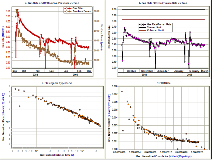
This case represents a well that was stimulated after three months of production. Some of the useful diagnostic plots are shown in Figure 2.

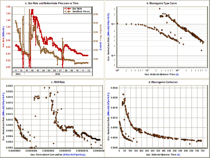
Figure 2a shows the rate and sandface flowing pressure versus time plot. From this plot, we can see that the well was shut in for two days in February 2005 and after that the rate and pressure increases rapidly. Looking at Figure 2b, it is evident from this plot that there are two stems in the typecurve. One stem is for data before February 2005 and one is for data after February 2005. It can also be seen that the productivity of the well (q / Δpp) has increased after February 2005. This is due to the fact that the well was fractured on February 5, 2005. Figure 2c is a plot of q / Δpp versus Gp / Δpp. Extrapolation of this plot to the x-axis gives an estimate of the original-gas-in-place. It is obvious from this plot that the frac not only improved the productivity of the well, but also added more reserves as shown by the increase from the original-gas-in-place to the ultimate-gas-in-place. Only data collected after February 5, 2005 should be used in any interpretation, as the reservoir model has changed.

Figure 2: Case 1 diagnostic plots

Case 2

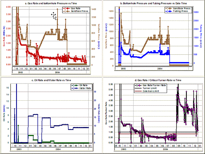
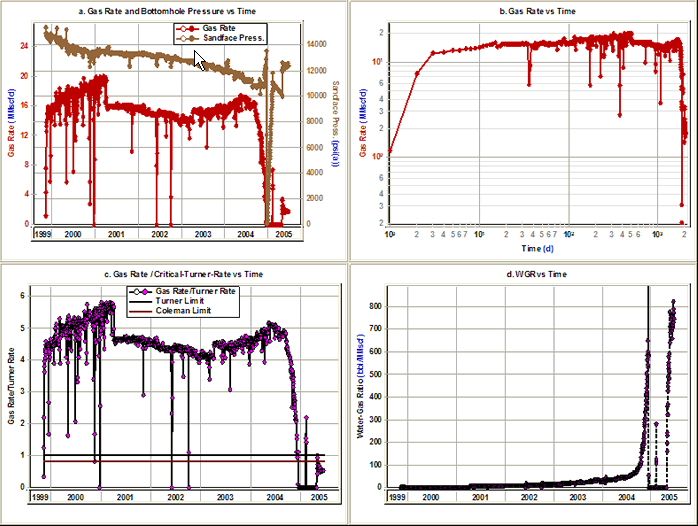
Figure 3a shows the gas rate and sandface flowing pressure versus time. It can be seen from this plot that the sandface flowing pressure is almost a straight line from the beginning of March 2004 until the middle of April 2004. The same thing can be seen for tubing pressure in Figure 3b. In practice, it is not likely that the tubing pressure profile would be a straight line for a period of time. If the tubing pressure has a straight line profile for a period of time, it implies that it was not measured frequently and the data has been interpolated and not measured. This will be reflected in the reliability of the calculated sandface flowing pressure data.

This well also produced water and oil. Figure 3c shows the oil rate and water rate versus time plot. Looking at this plot, it is obvious that the oil rate and water rate have flat profiles with large step changes. This again means that oil rate and water rate were not measured frequently and this will have a significant effect on the quality of the calculated sandface flowing pressure data, because multiphase flow calculations depend directly on gas-liquid ratios.

Figure 3d shows the gas rate / critical-Turner-rate ratio versus time plot. This plot shows that the well may be loaded by liquid from the beginning of March 2004 to the end of August 2004. This is consistent with fluctuations in the gas rate during this period. This plot also shows that the gas rate is higher than the critical-Turner rate from the beginning of September 2004 to the end. The tubing pressure during this period is constant and equal to 13.0 psi (apparently a gauge pressure of 0, converted to absolute). This is not a valid pressure. Therefore, the calculated flowing sandface pressure and the critical-Turner-rate calculations after September 2004 are not valid, and should be discounted in any interpretation.

Figure 3: Case 2 diagnostic plots

Case 3

Figure 4a shows the gas rate and calculated sandface flowing pressure versus time. Looking at this plot, everything seems to be normal. Figure 4b shows the ratio of gas-rate / critical-Turner-rate versus time plot. According to this plot, the rate is less than both the Coleman and Turner critical lift rates, which indicates that the well is probably loaded with liquids. However, there is no liquid production reported at all. The gas rate is higher than 2 MMscfd and there is no indication of slugging or liquid loading in the trend of the gas rate and flowing pressure. The Blasingame typecurve and FMB rate plots are well behaved. The problem in this case is that the specified tubing ID was wrong. This directly affects the values for critical-Turner rate, but has little effect on the calculated flowing sandface pressure, as it only affects the friction component of the pressure loss inside the wellbore, which is very small compared to hydrostatic pressure loss. Therefore, the flowing sandface pressures calculated using the wrong tubing ID, in this case of dry gas production, can still be used for analysis.

Figure 4: Case 3 diagnostic plots

Case 4

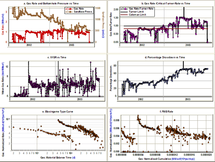
Figure 5a shows the gas rate and sandface flowing pressure versus time for a high permeability gas well. Figure 5b shows the ratio of gas-rate / critical-Turner-rate versus time plot for this well. This plot shows that the gas rate is lower than the Turner rate before July 1, 2002. Looking at the gas rate and sandface flowing pressure versus time and water-gas ratio versus time plot shows that something happened on July 1, 2002. There is a step change in the rate and the flowing pressure, and a significant increase in the water-gas ratio (Figure 5c). This behavior is consistent with a tubing change-out (where tubing is replaced with a smaller diameter to lift liquids and eliminate the liquid lifting problem). This tubing change was not documented for this well.

Looking at the Blasingame typecurve and FMB rate plots also shows there is some inconsistency between rate and flowing pressure data, as there are two stems on these plots. One of the stems is for data before July 1, 2002 and the other stem is for the data after July 1, 2002. The main reason for having two stems is because of having “stagnant” liquid column in the wellbore before July 1, 2002. This liquid column was not considered when calculating the sandface pressure during this period, and therefore, the calculated sandface pressure data for this part of data is wrong. Only data collected after July 1, 2002 should be used in any interpretation, as the calculated flowing sandface pressure data is more reliable.

Figure 5: Case 4 diagnostic plots

Case 5

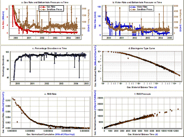
Figure 6a shows the gas rate and sandface flowing pressure versus time for a hydraulically fractured well. Figure 6 (that is, plots b-to-e) shows some of the proposed diagnostic plots. These plots do not show any inconsistency between rate and pressure.

Figure 6f shows the ratio of gas-rate / critical-Turner-rate versus time plot. According to this plot, the gas rate is less than the critical liquid lift rate throughout the whole producing life. In addition, Figure 6a shows fluctuation in gas rate and this indicates that there is slug flow. Although there is indication of slug flow in Figure 6a and liquid loading in Figure 6f, no water production has been reported. Therefore, sandface pressure calculations from wellhead pressure are likely incorrect.

Figure 6: Case 5 diagnostic plots

Case 6

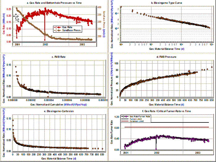
Figure 7a shows the gas rate and calculated sandface flowing pressure versus time for a horizontal gas well. Visual inspection of Figure 7a indicates some inconsistencies between pressure and rate. It can be seen from this plot that:

The pressure profile is flat from July 2002 to December 2002.
There is a step change in pressure at the end of July 2003, but this step change is not reflected in the gas- rate data.

Some of the proposed diagnostic plots are shown in Figures 7 b-f. There is no evidence of these inconsistencies in Figures 7 b-e. Figure 7f shows the plot of percentage drawdown [ (Δp / pi) * 100 ] versus time for this well. According to this plot, except for the first two months of production, the well is producing under almost 85% drawdown. This means that we are dealing with a high drawdown well, and that the rate is insensitive to flowing pressure and that any discrepancies in flowing pressure have very little effect on interpretation. This is the reason why no inconsistency was observed in Figures 7b-e.

Figure 7: Case 6 diagnostic plots

Case 7

This is a high-permeability gas well. This well is producing through tubing and only tubing pressure data is available. Figure 8a-f shows some of the diagnostic plots for this well. Figure 8a shows the gas rate and sandface flowing pressure versus time for this well. Everything seems normal except for the data between the beginning of May 2002 until the end of July 2002:

The sandface flowing pressure suddenly decreases in early May 2002, but this step change is not reflected in gas-rate data.
The gas rate suddenly decreases in late June 2002, but this step change is not reflected in the sandface flowing pressure data.

To find out why the rate and pressure are not consistent in this period, we reviewed at the water-rate data. The plot of water rate and sandface flowing pressure is shown in Figure 8b. This plot shows that the well was producing almost 50 bbl/d of water from the beginning of 2001 until the beginning of May 2002, and no water rate was reported from the beginning of May 2002 until the end of July 2002. The water rate affects both hydrostatic and friction pressure losses in the wellbore, and has a huge effect on the magnitude of the calculated sandface pressures. This can explain the inconsistency between rate and sandface pressure from the beginning of May 2002 until the end of July 2002, as the water rate is not reported. If the casing pressure had been available, the problem would have been less severe because the sandface pressure could have been calculated using casing pressure data instead. This would not have been affected by an incorrect liquid rate, as it involves a hydrostatic head calculation of a dry gas column to the end-of-tubing.

Figure 8c shows the plot of percentage drawdown versus time for this well. According to this plot, except for the first two months of production, the well is producing under almost 95% drawdown. This means that the diagnostic plots which use Δp or Δpp may not show any inconsistency between rate and flowing pressure data even when they are not consistent. Looking at Figures 8d-f does not indicate any sign of inconsistency, which was expected because of high drawdown.

Figure 8: Case 7 diagnostic plots

Case 8

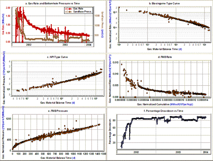
This is a high-permeability gas well. In this example, we do not emphasize the consistency between pressure and rate data. We just want to point out the value of diagnostic plots for indicating reservoir productivity issues. The gas rate and flowing sandface pressure versus time is plotted in Figure 9a. It can be seen from this figure that there are two step changes in rate, which are not reflected in pressure data. This plot also shows that the rate declines rapidly from September 2004. Figure 9b shows log q versus log t for this well. As can be seen, this log-log plot accentuates the declining trend in rate, as it compresses the late-time data. Liquid loading can sometimes cause this abnormal decrease in gas rate.

To investigate the possibility of liquid loading, the ratio of gas-rate / critical-Turner-rate is plotted versus time and presented in Figure 9c. It can be seen from this figure that when the gas rate started to decline, the gas rate was much higher than the critical liquid lift rate. The rapid decline in rate therefore indicates a decrease in reservoir productivity and not liquid loading. Figure 9d shows the water-gas ratio versus time for this well. This plot shows a rapid increase in the water-gas ratio at the same time that rate declines rapidly. Therefore, the rapid decline in gas rate was because of water reaching the well inside the reservoir and not liquid loading, and in fact, it is a reservoir problem not a wellbore problem. The fact that this well is producing this much water could mean that we are dealing with an active water-drive reservoir, or that a secondary gas cap is pushing water ahead of it to the well. The well was shut in for six months, but after that, the same problem occurred very quickly (that is, a high water-gas ratio).

Figure 9: Case 8 diagnostic plots

Case 9

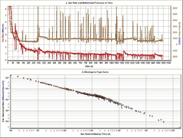
As mentioned earlier, the first step in production data diagnostics is the removal of outliers to eliminate any incorrect interpretation caused by these outliers. It was also mentioned that often outliers show a unit slope on typecurves. In this example, we present a dataset that shows this problem. Figure 10a shows the gas rate and sandface flowing pressure versus time. The outliers are shown by hollow points, so they can be distinguished from the rest of the data. Figure 10b shows the Blasingame typecurve plot for this case. The outliers are also shown by hollow points in this plot. It can be seen from this plot that the unit slope on this typecurve is caused by outliers, not depletion. Therefore, this unit slope should not be used as an indication of original-gas-in-place or boundary-dominated flow.

Figure 10: Case 9 diagnostic plots