The Fetkovich typecurves are applicable to wells that produce at constant sandface pressure. Many wells, particularly gas wells, experience a decline in sandface pressure during their life. Blasingame and his students / co-workers (McCray, Palacio) developed a time function that enables the matching of production rate data on Fetkovich typecurves, even when the flowing pressure is varying. After developing different time functions, they came up with a simple function they called "material balance time" which works very well when the change in sandface pressure is smooth, as is often the case in production operations. They, and Agarwal-Gardner et al., also demonstrated that using material balance time converts the constant pressure solution into the constant rate solution, which is the solution widely used in the field of well testing.
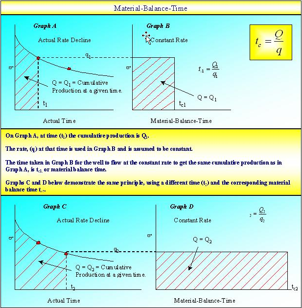
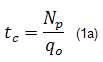
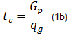
Conceptually, material balance time is defined as the ratio of cumulative production to instantaneous rate:

The symbol tc has been adopted as it represents a corrected time based on cumulative production. It is also similar to the corrected "Horner" time that is used in build-up analysis in well testing, for correcting the effect of a varying flow rate. It is the value of time that a well has to flow at the current rate in order to produce the same amount of fluid (and hence honor the material balance principle). In the figure below, the cumulative production is represented by the area under the graph. The definition of material balance time makes these areas the same.
Derivation of material balance time for slightly compressible systems focuses on the flow of liquids, and does not address the pseudo-time issues for gas reservoirs. It is fundamental to two basic ideas, namely the equivalence of constant pressure and constant rate solutions, and the harmonic stem of decline curves. Material balance pseudo-time for gas accounts for changing pressure-volume-temperature (PVT) properties with reservoir pressure.
Constant compressibility fluids
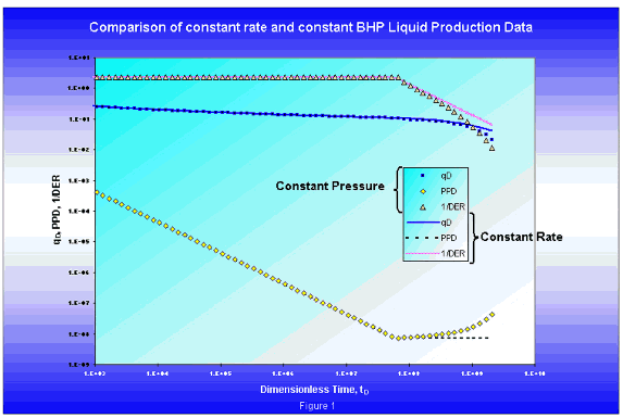
Consider an oil reservoir. A comparison of the constant rate (declining pressure) and constant pressure (declining rate) typecurves obtained when plotting against dimensionless time (based on area) shows the equivalence of the two solutions during the transient period, and their divergence during boundary-dominated flow.
Material balance time also normalizes production histories in which both the rate and the pressure decline, provided that both sets of data decline monotonically.
Another way to state the functionality of material balance time is to say that it is effective in normalizing any rate / pressure history, so that it looks like the constant rate solution, provided that the rate / pressure history does not contain any disturbances large enough to disrupt boundary-dominated flow. A disturbance that is large enough to disrupt boundary-dominated flow, such as a sudden (and significant) decrease in back pressure, would introduce a new transient flow period. Since material balance time is designed to normalize boundary-dominated flow only, it loses its effectiveness if a new transient is introduced.
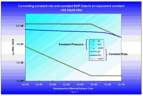
When the same typecurves (in figure 1) are plotted against dimensionless material balance time, the late time portion of the constant pressure overlays the constant rate solution precisely. This is an important result because it illustrates that the same diagnostic plots used in pressure transient analysis can be inverted and used for rate transient analysis, provided that the material balance time function is used.
From the above figure, it can be seen that the inverse logarithmic derivative behaves very similarly to the logarithmic derivative on a welltest typecurve. During transient (radial) flow, it has a constant value of 2 (1 divided by ½). Upon reaching boundary-dominated flow, the inverse logarithmic derivative falls off with a constant slope of 1 on the log-log plot. The primary pressure derivative has the opposite behavior to the inverse log derivative, in that it exhibits a slope of negative 1 during transient flow, and becomes constant during boundary-dominated flow. This follows from the fact that the pressure decline for a well produced at a constant rate has a constant slope on log-log paper, during pseudo-steady state.
The 1/pD (qD) data, for different combinations of re / rw, exhibit a fan of transient stems that converge into one harmonic depletion stem when plotted against dimensionless time based on area. If the data is plotted against a dimensionless time based on effective wellbore radius rather than reservoir area, the transient stems merge together while the depletion stems fan out.
The main difference in appearance between Agarwal-Gardner (A-G) typecurves and Fetkovich typecurves is that the depletion stems for A-G typecurves all collapse to the harmonic case. This follows from the fact that the A-G typecurve normalizes all rate and pressure solutions, so that they behave like the constant rate solution for slightly compressible fluids. Figure 3 shows the A-G typecurves for a vertical, unfractured well.
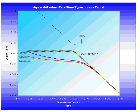
The presence of the inverse log derivative and pressure derivative plots on the A-G typecurve aids in the identification of transient and boundary- dominated flow regimes, in the same way that the logarithmic pressure derivative aids in flow regime identification on welltest typecurves.
Material balance time for oil
When analyzing oil wells:
The following development (see Palacio and Blasingame, 1993) applies rigorously to a system with constant compressibility, such as an undersaturated oil reservoir.
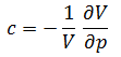
Using the definition of compressibility, the oil production from a reservoir is related to the drop in average reservoir pressure, as follows:

Separating the variables and integrating:
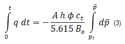
Recognizing that the left side is the cumulative oil production, the average reservoir pressure can be calculated from:
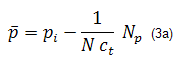
The important characteristic of equation (3a) is that it is always valid — regardless of time, flow regime, or production scenario (constant or variable flow rate). This is because equation (3a) is a material balance equation.
Note that if p is plotted vs. Np, then a straight line of slope 1/Nct and intercept pi is obtained. Of course, p is typically not available in practice, so we must use an alternate approach to applying this concept. Before doing so, we recast equation (3a) by including the definition of tc, as in Equation (1a):
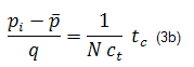
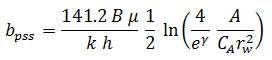
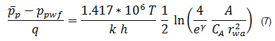
The second equation to be used is the steady-state solution for single-phase liquid flow in a rectangular reservoir containing a vertical well:
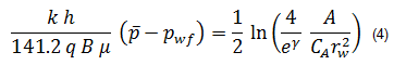
where:
γ = Euler's constant = 0.57721
Although equation (4) was derived for constant rate (variable pwf), Blasingame and Lee (1986) showed that it is also valid when the sandface pressure is constant (variable rate). Combining the material balance equation (3b) and the steady-state flow equation (4) gives:
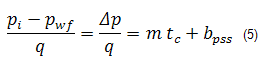
where:

and:
Equation (5), called the pseudo-steady state equation, suggests that a plot of Δp / q as a function of material balance time yields a straight line. If we assume q is constant, then equation (5) reduces to:
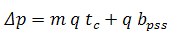
and a plot of ∆p vs tc yields a straight line.
Blasingame and Lee state that the importance of equation (5) is that it is also valid for moderately changing flow rate and sandface pressure conditions, so long as the transients caused by the changing inner boundary condition do not obscure the boundary-dominated flow behavior. In particular, equation (5) is directly related to two concepts: the equivalence of the constant pressure and constant rate solutions, and the harmonic stem of decline curves.
Material balance pseudo-time for gas
The application of material balance time to gas is more complex than it is for oil because of the varying PVT properties of gas. Accordingly, the simple concept of material balance time given by:
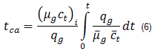
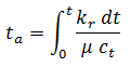
has limited application, and is considered to be only an approximation of the more rigorous formulation, which must be defined in terms of pseudo-time, ta. Material balance pseudo-time, tca, is defined as follows:
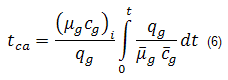
Equation (6) can be coupled with the steady-state flow equation for the flow of single-phase gas (which is the gas equivalent of equation (4) of this section), to give:
where:
γ = Euler's constant = 0.57721
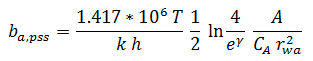
Addition of equations (6) and (7) results in the following equation:
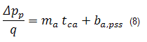
where:
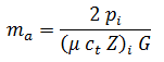
and:
Total compressibility
The definition of material balance pseudo-time described in equation (6) accounts only for the compressibility of gas. This is often a reasonable approximation as gas compressibility is typically much larger than that of liquid or rock. However, in some cases, the compressibilities of other fluids cannot be ignored. Thus, we require a more general definition of pseudo-time that accounts for the total system compressibility. Total compressibility includes gas compressibility, as well as water influx and production, formation and residual fluids compressibilities, and gas desorption.
The following is a derivation for total compressibility in a general form.
Material balance equation
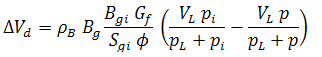
Refer to material balance analysis theory - gas material balance for the general gas material balance equation. The general gas material balance equation can be expanded to include water influx and production, formation and residual fluids compressibilities, and desorption of gas (∆Vwip, ∆Vep and ∆Vd, respectively) as follows:
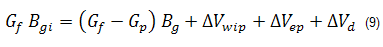
where:
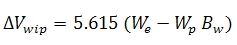
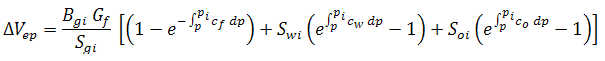
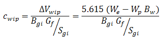
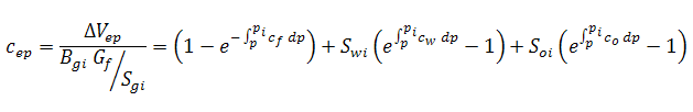
The relative change of the pore volume due to water influx and production, formation and residual fluid expansion, and desorption of gas (cwip, cep, and cd, respectively), can then be defined as:
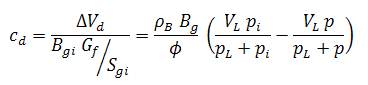
If the adsorption saturation correction has been enabled, cd is modified as follows:

For more information, see material balance analysis theory - advanced gas material balance.
Solving for total compressibility (ct)
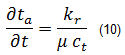
The solution for total compressibility comes from the definition of pseudo-time:
By taking the partial derivative of pseudo-time with respect to time, total compressibility is exposed:
The following chain rule of derivatives is applied:
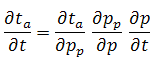
Therefore, equation (10) may be expressed as:
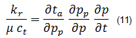
Note that the inclusion of a permeability term in the above definition of pseudo-time accounts for a pressure-dependent permeability. For more information on theory and equations, see geomechanical reservoir models.
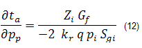
Solving for ∂ta / ∂pp
Defining pseudo-pressure:
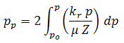
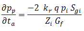
Relating pseudo-pressure to pseudo-time (Rahman et al., 2006):
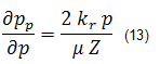
Solving for ∂pp / ∂p
From the above definition of pseudo-pressure:
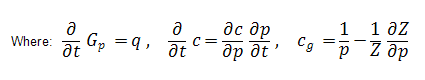
Solving for ∂p / ∂t
Dividing both sides of equation (9) by (Gf Bgi / Sgi) and recalling that Bg = (psc Z T) / (Tsc P):
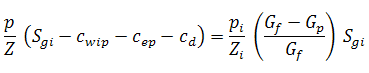
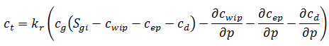
Letting c equal the summation of cwip, cep, and cd; and rearranging:
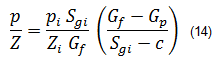
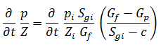
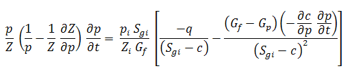
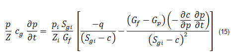
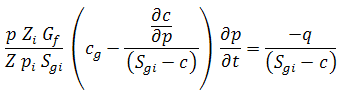
Rearranging equation (14) such that:
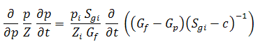
Equation (15) can now be written as:
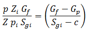
And then solved for ∂p / ∂t:
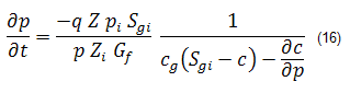
Substitution
Equations (12), (13), and (16) are substituted into the chain rule of derivatives from equation (11) and simplified:
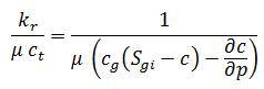
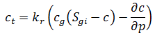
As c equals the summation of cwip, cep, and cd: