Numerical URM

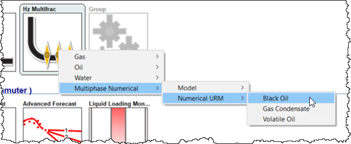
We recommend reviewing the methodology summary prior to conducting this analysis for the first time. The numerical unconventional reservoir module (URM) worksheet is accessible by clicking the Hz Multifrac thumbnail.

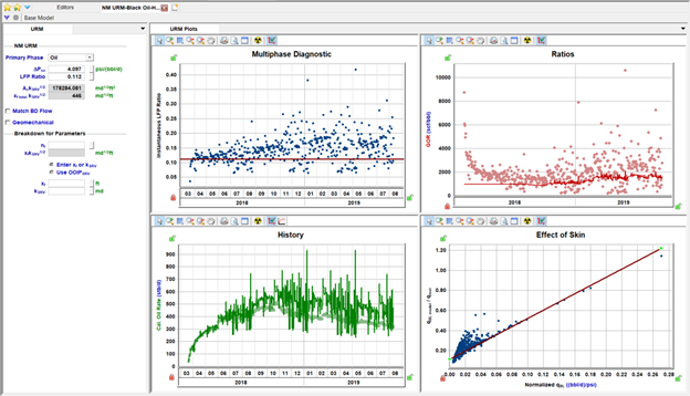
In a newly created worksheet, only the History plot and Ratio plot are populated, showing the historical data for the well.

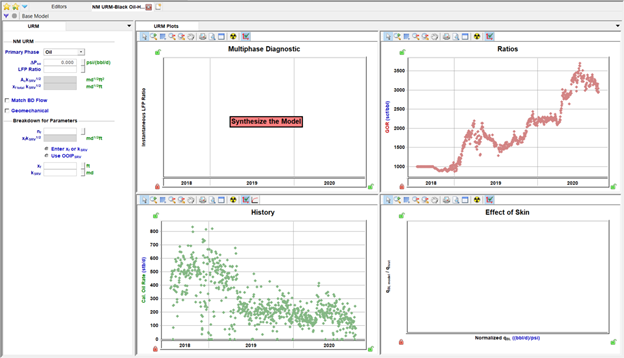
To begin, click the Synthesize icon () to run the base model, which is used to calculate the data points displayed in the Multiphase Diagnostic and Effect of Skin plots. The History and Ratios plots also display a synthetic line generated from the base model results.

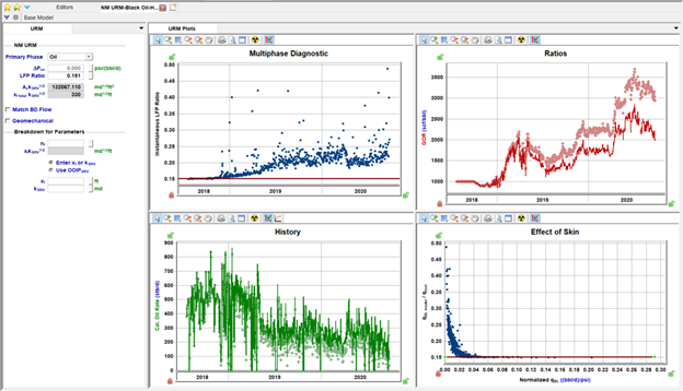
To use numerical URM, start with the Multiphase Diagnostic plot. The horizontal line on this plot represents the linear flow parameter (LFP) ratio used to determine A_c√k_SRV and starts as a fit of the first 25% of the data. Adjust this line on the plot, or type a new value for the LFP ratio to match the flat portion of your data points. When this is matched, the synthetic lines on the History and Ratios plots should also look like a good match to your data during the linear flow portion (the duration that is flat on the Multiphase Diagnostic plot).

If you are only interested in analyzing the linear flow data, you can now type the n_f in the Breakdown for Parameters section and type either x_f or k_SRV to have the other calculated from A_c√k_SRV. This can then be used in models or for other analyses.

We recommend starting your analysis with ΔP_s = 0 (no additional pressure drop) and leaving the analysis line on the Effect of Skin plot flat. However, additional pressure drop can be accounted for if:

A declining trend is observed in the early-time data of the Multiphase Diagnostic plot, and
Points on the Effect of Skin plot follow an increasing straight-line trend

To account for additional pressure drop:

1. Adjust the straight line on the Effect of Skin plot, or change the value of ΔP_s to match the trend.

2. The Multiphase Diagnostic plot adjusts accordingly (the decreasing trend at the beginning should flatten) — adjust the horizontal LFP line on this plot, if needed.

3. The synthetic line on the History plot also adjusts — check if the match is good, both at the early flow and during the first linear flow.

Note: Real data is usually scattered on the Effect of Skin plot. As a result, identifying a straight line with a positive slope can be quite challenging.

Without ΔP_s:

With ΔP_s:

If data is too scattered and the match is non-unique on the Effect of Skin plot, use the Multiphase Diagnostic plot and make sure the flat line is fitted through the transient linear flow portion of the data.

As a result of accounting for the additional pressure drop, you may get more accurate result for the A_c√k_SRV value. This also indicates that you need to use a lower fracture conductivity in order to model the dataset numerically.

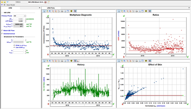
Matching boundary-dominated flow

If your data shows a clear transition out of linear flow, you may want to match the later data with an A_SRV or OFIP_SRV. Start by selecting the checkbox for Match BD Flow so the inputs are displayed. You can click the View Defaults and Limits buttons () on the right of the input fields to pull A_SRV or OFIP_SRV from other analyses, such as FMB. You can also directly type a value and the other value is calculated. After A_SRV or OFIP_SRV are populated, click the Synthesize icon () to calculate a boundary-dominated match from the base model. A synthetic line is displayed on the Multiphase Diagnostic plot, and the History and Ratios plots have synthetic lines based on the boundary-dominated match.

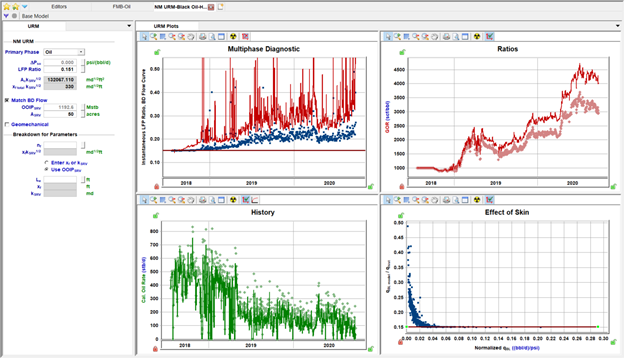
The synthetic line on the Multiphase Diagnostic plot is a good indication of the quality of the boundary-dominated match. If the synthetic line is above your data, try a larger A_SRV or OFIP_SRV. If the synthetic line is below your data, try a smaller value.

Better match:

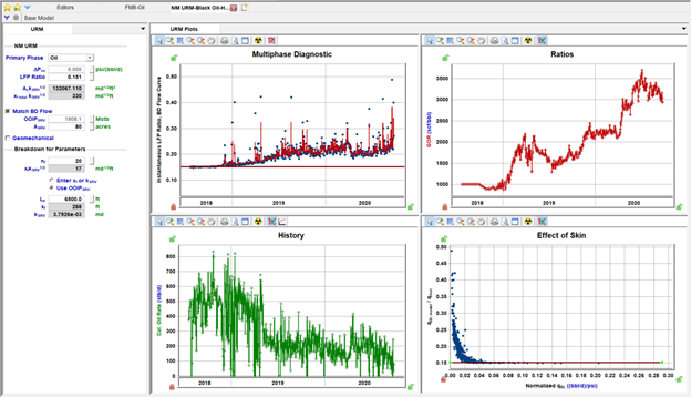
Similar to the linear flow match, after you are satisfied with the match to your data, you can populate the inputs in the Breakdown for Parameters section to get specific results. When Match BD Flow is used, the L_e for your well can be used in combination with the A_SRV to calculate both x_f and k_SRV.

Other settings

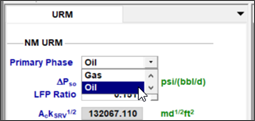
Numerical URM defaults to a Primary Phase of Oil for Volatile Oil, Black Oil when there is oil production, and to a Primary of Phase of Gas for Gas Condensate. When there is no oil production for the Black Oil model, Harmony Enterprise sets the Primary Phase to Gas. You can switch the primary phase between oil and gas. The OFIP_SRV below Match BD Flow and data on the plots is based on the Primary Phase selection.

There are also options to enable the geomechanical and adsorption (for gas only) model options. These use the parameters specified in the Properties editor.

If you want to view or modify the base model, it can be displayed by clicking the Base Model button in the toolbar, which displays a tab for the base model parameters and plots:

The base model primarily uses inputs from the Properties editor with a subset of inputs that you can modify. The Base Model Plots display the rates, ratios, and synthetic reservoir pressure from the base linear model.

If you change base model inputs and want to revert to the default settings, click the Reset to Default Values button. The phases enabled in the base model are based on production data from the well.

In addition to the base model parameters, gridding for the model can be viewed or modified in the Options tab, which defaults to coarse gridding for faster performance. You can refine the gridding, but running the base model is slower.

Non-SRV cases

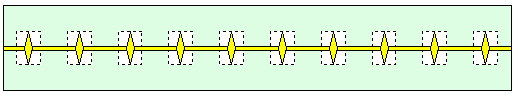
The numerical URM analysis is best-suited for analyzing wells that can be modeled using stimulated reservoir volume (SRV) geometry. However, if you believe that the well can be better described using enhanced-fracture-region (EFR) geometry (see image below), numerical URM analyses can still be useful.

Analyzing the linear portion of the flow for this case can be done in the same way as described above. You can:

Estimate A_c √k
Enter h, n_f, and x_f to find k (based on these entered parameters and estimated A_c √k)
Enter h, n_f, and k to find x_f (based on these entered parameters and estimated A_c √k)
Estimate t_elf based on where the points start curving upward

However, matching the boundary-dominated portion of data cannot be done in the same way.

If data clearly indicates t_elf, you can create a base boundary-dominated model with the same t_elf to find the OFIP_SRV. However for this geometry, the "use OFIP_SRV" option in the Breakdown for Parameters section should not be used as A_SRV = 2x_f * L_e is not true for this case.

Note: In this case, we do not expect the boundary-dominated portion of data to match. This is because the horizontal multifrac model experiences true boundary-dominated flow, while the actual well experiences transition; there is no true boundary and some contribution from the matrix affects the behavior after the t_elf.