Numerical model theory

Background

There are two main types of models used to simulate the flow of fluid through porous media: analytical models and numerical models. Both types have their advantages and disadvantages.

Analytical models

Analytical models have relatively short calculation times, so you can history match with these models quickly. More than that, you can even match the model automatically using automatic parameter estimation (APE).

The main disadvantage for these models is that they can only simulate single-phase flow – either liquid or gas, but not gas and liquid flowing together. Additionally, analytical models do not fully account for changing fluid properties with pressure. In case of liquid flow, fluid properties are assumed to be constant, and in case of gas flow, the change of fluid properties with pressure is accounted for by using pseudo-pressure and pseudo-time.

Unfortunately, pseudo-time is not an exact transformation. As a result, changing gas properties are only accounted for to a certain extent. Therefore, in cases where pressure varies significantly across the reservoir (for example, pays with low permeability), long-term forecasts for gas analytical models may be inaccurate. There is no known way to fully account for the change in fluid properties when using analytical models.

Numerical models

The numerical models have been significantly improved in Harmony Enterprise. One of the key benefits is the improvement in computation time, so that the model runs almost as fast as an analytical model. These modifications include:

using the pseudo-pressure formulation
optimized "gridding" — by using the pseudo-pressure formulation, you can use larger grid cells without affecting the accuracy of calculation results; using larger grid cells also makes calculations run faster.

With numerical models, you can model multiphase flow, and account for changing properties of each phase, and the interaction between phases.

The main disadvantage for these models is their long computation time. With the numerical model, the reservoir is divided into a number of cells, and then the flow is modeled simultaneously in all cells. To be able to assume constant pressure and constant fluid properties within each cell, the size of each cell needs to be relatively small. Therefore, the number of cells required for an accurate solution becomes large, which results in a long computation time. Note that decreasing the number of cells to reduce computation time may significantly affect calculation results.

Performing a manual history match for numerical models is time consuming. In addition, an automatic history match for numerical models is complicated, and thus not widely available in commercial software.

General formulation for the single-phase model

To calculate pressure across the reservoir, we divide it into a number of grid cells. At each timestep (n+1), we formulate a material balance for each cell.

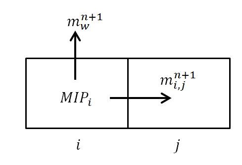
To define components of mass balance for cell i at timestep n+1:

Mass in place (MIP) for cell i at timestep n+1 can be calculated as:

Equation 1

where:

V_bi = bulk volume for cell i

p_iⁿ⁺¹ = pressure for cell i at timestep n+1

φ = porosity

ρ = density

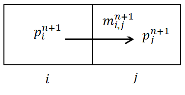
Mass flow from cell i to the adjacent cell j during timestep n+1 can be calculated as:

Equation 2

(We used Darcy’s Law to calculate flow rate.)

In equation 2:

= flow rate from cell i to cell j at timestep n+1

A_i,j = cross-section area between cells i and j

L_i,j = distance between the centers of cells i and j

μ = viscosity

k = permeability at the initial pressure

k_m(p) = permeability multiplier (permeability at a certain pressure is calculated as ).

Mass produced at the well during timestep n+1 (if well penetrates cell i) can be calculated as:

Equation 3

where:

WI = wellbore index (as per Peaceman 1978 or Babu and Oden, 1989)

= pressure at the wellbore at timestep n+1

Material balance for cell i at timestep n can be written as:

Equation 4

Using equations 1, 2, and 3, and bringing all the terms to the left, we can rewrite equation 4 as:

Equation 5

Assuming that the pressure distribution has been calculated for timesteps 1, 2, ... n, to calculate pressure distribution at timestep n+1, we formulate material balance (equation 5) for each cell, and solve all these equations simultaneously. Unknowns of the system are for each cell i; therefore, the number of equations is the same as the number of unknowns, and the system can be solved.

Well constraint considerations

For a well producing at a specified sandface pressure, the described system of equations can be used directly (because is known). However, for a well that produces at a specified surface q, an extra equation is required.

Equation 6

where:

i = summation index for all cells penetrated by the well

ρ_sc = fluid density at standard conditions

TPC stabilization

Tubing performance curve (TPC) stabilization is applied when the deliverability of the model intersects with the well’s TPC curve at a point where the slope is negative (found at low rates). This portion of the TPC is generally characterized by unstable, slugging flow.

When the resultant operating point is found to be in this unstable section, the numerical model can respond with a series of shut-ins and intermittent production.

TPC stabilization switches the forecast reference point from wellhead to sandface, allowing the forecast to continue with a constant sandface pressure equal to the minimum sandface pressure of the TPC.

This stabilization can be deselected in the Options dialog box, Numerical node.

Considerations when estimating fluid properties

In the above formulation, we use rock and fluid properties estimated at certain pressures. The term is used in (equation 2) and in (equation 3).

Some logical questions are:

At what pressure should we estimate this term?
Should we use pressure in one of the cells, or some kind of average?

Fluid properties may significantly vary with pressure (especially if the modeled fluid is gas); therefore, selecting the correct way of estimating properties becomes important.

In classical numerical simulation (including numerical models in single-user Harmony), properties are estimated at the pressure of the upstream cell (that is, the cell with the higher pressure). For such a simulation to be accurate, you should ensure that properties in the adjacent cells are close. To achieve this, grid cells have to be small enough. Unfortunately, having smaller grid cells results in longer computation times.

With the numerical model in Harmony Enterprise (both for single-well and multi-well), we use the pseudo-pressure formulation to estimate fluid properties and calculate mass transfers.

Numerical model pseudo-pressure definition

The numerical model pseudo-pressure is defined as:

Equation 7

Note: For gas, the definition of numerical model pseudo-pressure is very similar to a traditional pseudo-pressure. To see this, express density as (z = gas compressibility factor, T = temperature, R = gas constant, M = molar mass). This results in the following equation:

Equation 8

Therefore, the numerical model pseudo-pressure and traditional pseudo-pressure are different by a constant factor.

Numerical model pseudo-pressure formulation

As was mentioned in considerations when estimating fluid properties, the calculation of mass flow from one cell to another given in equation 2 has a deficiency: it does not account for a variation of fluid properties with pressure. The numerical model formulation modifies equation 2 to get a relationship between the mass flow rate and pressure drop when properties are changing with pressure.

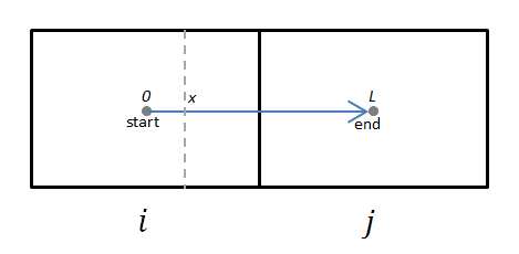
At each cross-section at any given distance (x), the pressure gradient across the cross-section can be expressed using the differential form of Darcy’s Law:

Equation 9

where is the mass flow rate across the cross-section. This can be rearranged as:

Equation 10

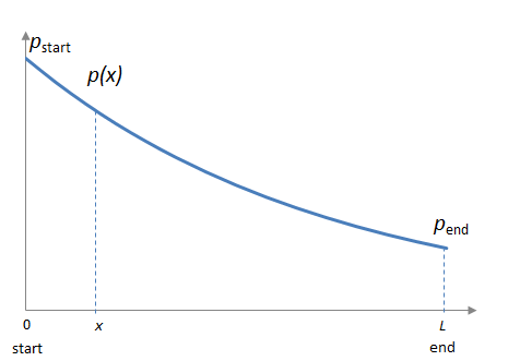
Integrating both parts from 0 to L with respect to x, and using the left-side of the equation is a constant with respect to x, we get the following equation:

Equation 11

Note: We used the definition given in equation 7 for the last transformation.

To summarize, when fluid properties are changing with pressure, the mass flow rate through the cross-section can be calculated as:

Equation 12

Therefore, equation 2 can be modified to account for changing properties. The mass flow from cell i to cell j during timestep n+1 is calculated as:

Equation 13

Equation 3 can be modified in a similar fashion. Mass produced at the well during timestep n+1 is calculated as:

As a result, the material balance equation for each cell (equation 5) is modified to:

Equation 14

Assuming that the pressure distribution has been calculated for timesteps 1, 2, ... n, to calculate pressure distribution at timestep n+1, we formulate a modified material balance (equation 14) for each cell, and solve all these equations simultaneously. Unknowns of the system are for each cell i; therefore, the number of equations is the same as the number of unknowns, and the system can be solved.

Note: Well constraints are treated in a similar way to general numerical model formulations.

Modifications for the multiphase model

In the case where there are two or three phases flowing together, the multiphase solution follows similar logic as single-phase flow, with a few modifications.

The mass balance equation (equation 4) has to be modified to account for the fact that fluid can change from one phase to another (e.g., oil can evaporate and become gas, or gas can condense to liquid).
In the single-phase case, the mass balance equation is written for each cell; therefore, we get n equations (where n is the number of cells). In the multiphase case, the mass balance equation is written for each cell for each phase; therefore, we get n•"number of phases" as equations.
In the single-phase case, the unknowns of the system are pressures in each cell; therefore, we get n unknowns. In the multiphase case, the unknowns of the system are pressures in each cell (n), and saturations for each cell; therefore, we get total n•"number of phases" as unknowns. (We use the fact that the sum of all saturations is equal to 1 for any of the grid cells.)
When calculating a mass transfer from one cell to another (equation 2) and a mass transfer from the cell to the well (equation 3), we have to account for relative permeability.
For the single-phase case, we re-write the mass transfer term in terms of pseudo-pressure (equation 13). In the multiphase case, we can do the same thing, but there will be different pseudo-pressure functions for different phases. (The pseudo-pressure formulation for each phase follows the definition given in equation 7, but ρ, μ, and k are different for different phases.)
For the single-phase case, the system of equations can be solved in terms of pseudo-pressures (the unknowns are pseudo-pressures in each cell). For the multiphase case, equations have to be solved in terms of pressure (the unknowns are pressures and saturations in each of the cells). The pseudo-pressure formulation is only used to calculate mass transfer between cells.

Advantages of using the pseudo-pressure formulation

Pseudo-pressure formulation makes simulation significantly faster than classical numerical simulation modeling for the following reasons:

1. Smaller number of grid cells: In classical numerical simulation, grid cells have to be small enough to consider constant fluid properties within each cell. Pseudo-pressure formulation accounts for a variation of fluid properties between the centers of two adjacent cells; therefore, it is possible to have larger grid cells. By having a smaller number of grid cells, calculation speed increases.

2. Faster solution for a non-linear system: While performing numerical modeling, equation 5 is solved at each timestep. This system of equations is non-linear; therefore, it is solved iteratively, using the Newton-Raphson method. This method involves calculating derivatives of each matrix element with respect to each unknown. Calculating these derivatives is faster for pseudo-pressure formulation (equation 14), because we have to deal with one fluid property function () as opposed to a combination of three functions () for traditional formulation. More than that, due to the integral nature of , its derivative is calculated easily.

Modifications for multi-well models

Multi-well models in Harmony Enterprise are multi-phase numerical models. They use the same calculation engine and the same formulation as is used by single-well numerical models that is described above. However, the gridding is adjusted to include multiple wells and gridding is done differently for different completion types.

Since multi-well models allow multiple layers, additional modifications are made to model flow in a vertical direction, and to model layers that are connected through the wellbore.

Modifications for flow in a vertical direction

Re-writing Equation 2 for each phase individually, the mass flow rate of phase x from cell i to the adjacent cell j during a particular timestep, can be calculated as:

Equation 15

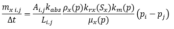
Where k_rx is a relative permeability and the remaining variables are the same as defined in Equation 2.

To account for the fact that the direction of flow may have a vertical component, the equation should be adjusted as:

Equation 16

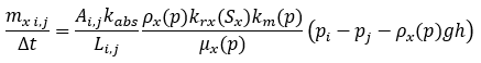
Where h is a vertical distance between the centers of cells i and j.

Note: If the direction of flow is horizontal (h=0), Equation 16 reduces to Equation 15. When there is no flow in the system, Equation 16 reduces to: p_i - p_j = ρ_xgh. In other words, each phase is in hydrostatic equilibrium.

Modifications for modeling layers connected through the wellbore

The conventional multi-well (CMW) model enables you to model layers that are connected only through the wellbore. In this case, the model has equations for all of these cells solved simultaneously:

Reservoir cells in each of the layers (marked as rectangles with a thin black outline)
Cells representing the wellbore (marked as rectangles with a thick blue outline)

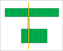
Reservoir cells are connected to each other and the flow rate through each connection is governed by Equation 16.

Reservoir cells are also connected to wellbore cells and the flow rate through each connection is governed by Equation 16, using the wellbore index WI, instead of:
.

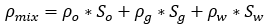
Wellbore cells are also connected to each other, but this connection is different, because flow in this connection represents flow of the fluid in the pipe, not in the porous media. Phases inside the wellbore are assumed to be mixed and to flow as a single homogeneous fluid.

Based on a fully mixed assumption, the density of the mixture is calculated as:

Equation 17

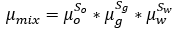
And viscosity of the mixture is calculated as:

Equation 18

The volumetric flow rate of the mixture is then calculated as per Darcy’s law:

Equation 19

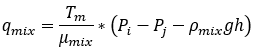
Where T_m is a high number to represent the high conductivity of the pipe.

This rate can then be split into rates for individual phases:

Equation 20

Note that since T_m is a very high number, Equation 19 results in this pressure drop across the pipe segment:

Equation 21

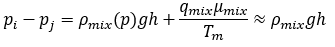
Therefore, pressure drop across the wellbore calculated using this approach approximately equals the hydrostatic pressure drop for a homogeneous mixture.