Pressure loss calculations in multilayer wells

This topic describes the underlying logic for multilayer wellbore pressure calculations. For step-by-step instructions on how to set up multilayer wells, see analyze well data. For information on what a multilayered well is, see multilayered wells.

For wells with multiple layers, pressure calculations can only be performed in the Production editor under the following scenarios:

• Flow path = casing; Pressure source = casing or gauge
• Flow path = tubing; Pressure source = casing, tubing, or gauge
• Flow path = annulus; Pressure source = casing or tubing
• Flow path = gas lift (tubing or annular); Pressure source = tubing or casing

The underlying logic for pressure-drop calculations is essentially the same for both multilayer and single-layer wells. However, multilayer wellbore calculations are somewhat more complicated than single layer since different layers (formations) can produce at different rates.

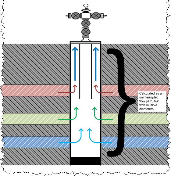
Note:    There is no limit to the number of layers in a multilayer well. For simplicity, the figures below generally show no more than three layers, but the logic holds for any number of layers.

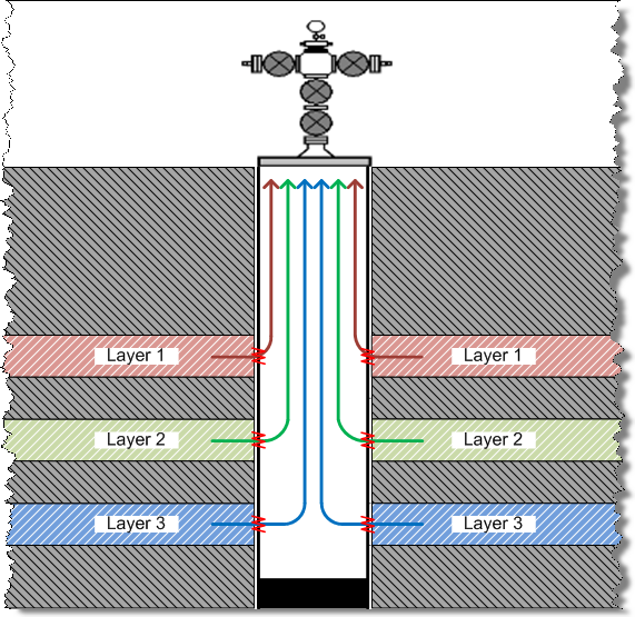
As can be seen in the figure above, the rates from all layers are summed in the wellbore, but only when each layer is encountered. Consequently, the combined rates from all three layers are used to calculate the pressure drop from the wellhead to Layer 1. However, to calculate the pressure drop from Layer 1 to Layer 2, only the rates from Layer 2 and 3 are required. Furthermore, only the rates from Layer 3 are required to calculate the pressure drop from Layer 2 to Layer 3.

In most cases, the production from each layer is similar (for example, each is producing some proportion of gas, oil, and water). For these common situations, the logic is relatively straightforward, with the wellbore containing the same overall fluid composition from top-to-bottom, with the rate dropping as each layer is passed, and the production from that layer is removed. However, it is possible for each layer to produce a unique type of fluid – for example, one layer flowing only gas, a second layer flowing only water. When this situation occurs, then the logic can become more complicated. The rest of this help topic describes this logic in depth.

Note:   Only fluid properties specified at the well level are used in wellbore pressure calculations. If properties are entered on a per-layer basis, they are not used in the wellbore pressure calculations, but instead are used in analyses created against that layer.

Fluid combinations

When mixing fluids, three possible rates are considered: gas, oil, and water. In addition, any or all of those rates can be zero, creating eight possible fluid combinations per layer. Thankfully, not all of those combinations require a unique method to calculate pressures. In fact, only three calculation methods are necessary:

1. Single-phase gas

2. Single-phase liquid

3. Multiphase (gas and liquid combined)

Note:   These methods are described in pressure loss calculations.

In the multilayer example above, there are three layers producing into the wellbore; this is the simplest scenario, since the example wellbore has no tubing installed. If tubing exists in the wellbore, then additional considerations must be made. The following sections are broken out to describe the specific logic required based on the existence of tubing, and the direction of flow.

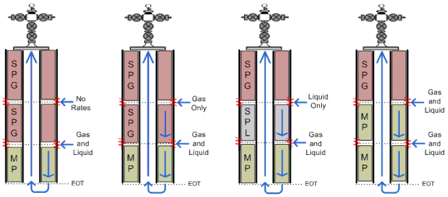
Examples: calculations when no tubing is present (casing flow only)

Pressure calculations within the casing string always assume that the direction of flow is towards the wellhead. The type of calculation performed (for example, single phase or multiphase) depends upon the constituent fluids within the wellbore. The following figure, with four different scenarios, shows the type of calculation required for each combination of inputs into the wellbore.

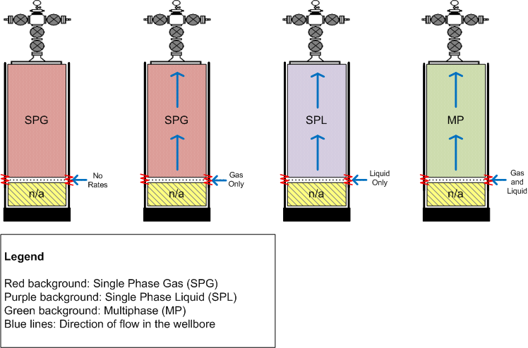
While the figure above only accounts for a single layer, it is useful as a reference case when further layers are considered. When additional layers are encountered, then the rates are summed to determine whether a single-phase gas, single-phase liquid, or multiphase calculation is required. However, a key difference exists when the deepest layer is shut in (no rates) – in such a case, the software examines all the layers above the deepest layer to determine whether there will be a column of static gas, or static liquid. The rules governing this are described in Group D.

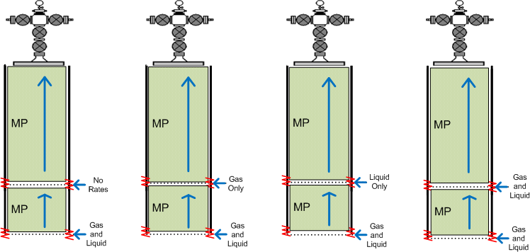
The following figures describe the logic that is used when there are two layers below end of tubing (EOT). This logic can be extrapolated for application to any number of layers.

Group A: deepest layer flowing gas & liquid

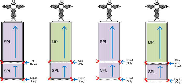
Group B: deepest layer flowing liquid

Group C: deepest layer flowing gas

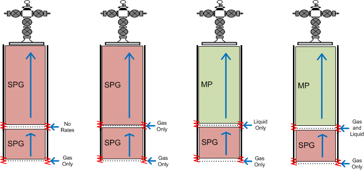
Group D: deepest layer not flowing (shut-in)

When the deepest layer is shut in (zero rates), then a static column exists from the bottom of that layer up to the next flowing layer. This static column must be gas or liquid. The logic applied is as follows:

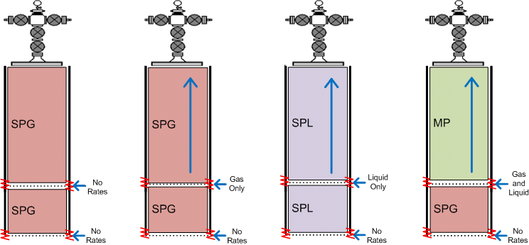
One key assumption is that if gas and liquid are produced from a single layer, then the gas carries that liquid upwards. If liquid loading is suspected, it can be analyzed using other methods (for example, Turner's equation).

Note:   When calculating pressure at the overall well datum (Well MPP), a shut-in layer is presumed for calculation purposes.

Examples: calculations when tubing is the flow path

When tubing exists, and it is the flow path, we assume that the produced fluids travel up the tubing as soon as they are able to. Therefore, it follows that EOT forms an imaginary dividing line for the wellbore, so the overall calculations can be divided into two sections:

1. Calculations for all layers above EOT

2. Calculations for all layers below EOT

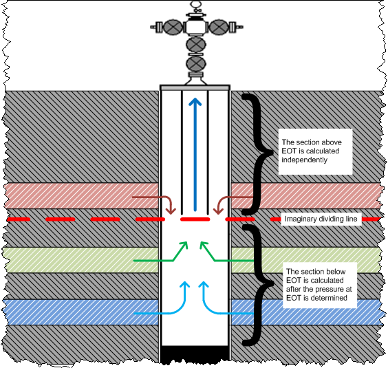
The examples below are categorized according to these two sections.

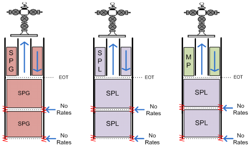
Examples: calculations for all layers above EOT

Calculations from the wellhead to EOT must always be performed, even if there are no layers above EOT. However, the order of events that takes place depends greatly on the pressure source chosen.

1. If the pressure source is "tubing", then the pressure at EOT is calculated first. This is done via the tubing path, using the total rates measured at surface. Once EOT pressure is known, then the pressure for each layer above EOT is calculated one at a time, following the annulus flow path.

2. If the pressure source is "casing", then the calculations follow the annulus flow path exclusively. From the surface down to the first layer, a static gas column is assumed to exist in the annulus. From the first layer down, the specified rates are used to calculate the pressure at the subsequent layer. On the other hand, if there is no layer between surface and EOT, then a static gas column is assumed throughout.

The following figure shows the possible fluid arrangements when a single layer exists above EOT:

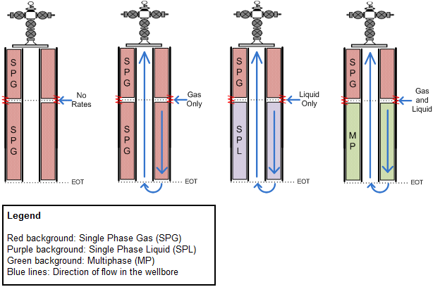
When additional layers are added to the system, then the rates must be combined in the order that they appear. For example, if a layer that was only flowing gas was followed by a layer that was only flowing water, then there would be a mix of gas and water at the second layer. This mix of gas and water would require a multiphase correlation to solve the pressure drop.

The following use cases show how rates would be mixed, if there were two layers above EOT. If more than two layers existed, then the same logic would be extended, with each subsequent layer experiencing the sum of the rates from the previous layers.

Group E: layer closest to EOT flowing gas & liquid | use cases 1 - 4

Group F: layer closest to EOT flowing gas only | use cases 5 - 8

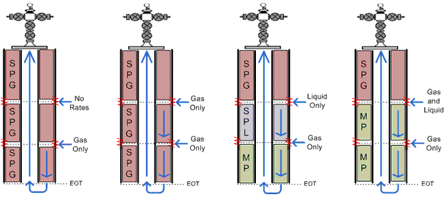
Group G: layer closest to EOT flowing liquid only | use cases 9 - 12

Group H: layer closest to EOT shut-in (no rates) | use cases 13 - 16

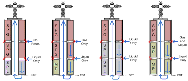
Examples: calculations below EOT

Pressure calculations for depths below EOT are nearly identical to the casing flow calculations described above. One minor difference is that the pressure and temperature at EOT are used as a starting point for all subsequent pressure calculations. The other difference is that there are additional rules for when all the layers below EOT are shut in.

Group I: deepest layer shut-in + all layers above shut-in

If every layer below EOT is shut in, then we must examine the flow conditions above EOT to determine the static column.

When all the layers below EOT have no rates, then the commingled rate for the layers above EOT must be examined. If there is any liquid production at all, then a static liquid column is assumed to exist from EOT to bottomhole. If there is no liquid production, then a static gas column is assumed.

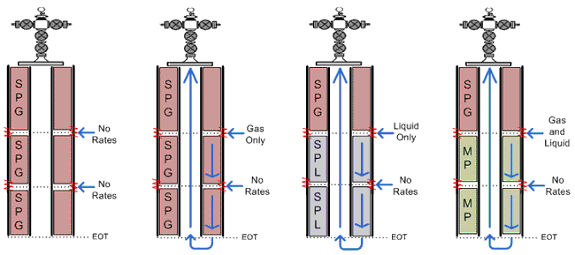
Examples: calculations when the annulus is the flow path

When tubing exists, and the annulus is the flow path, all the produced fluids are assumed to travel upwards (similar to the situation when there is no tubing in the wellbore). In fact, the logic for annulus flow is almost identical to that of casing-only flow, with the major difference being the calculation of friction. Consequently, the logic examples shown in casing flow examples also apply to annulus flow.

Pressure source considerations

There are two pressure source considerations, which are described below.

Flow path = annulus, pressure source = casing

When the pressure source is the casing (annulus) wellhead pressure, then the order of events is to start at the wellhead and then calculate the pressure for each successive layer down. The only difference for layers above and below EOT is the actual diameter used. For additional information, see annular diameters.

Flow path = annulus, pressure source = tubing

When the pressure source is the tubing head pressure, then the mandatory first step is to calculate the pressure at the EOT. Once EOT pressure is known, then pressures can be calculated at any layer either above or below EOT.