Superposition Time
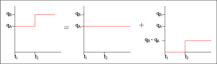
Superposition time is required in order to analyze variable rate tests. Superposition in time involves breaking up a multi-rate sequence into a set of single rates. The rate used for each step is the difference between the current rate and the previous rate.
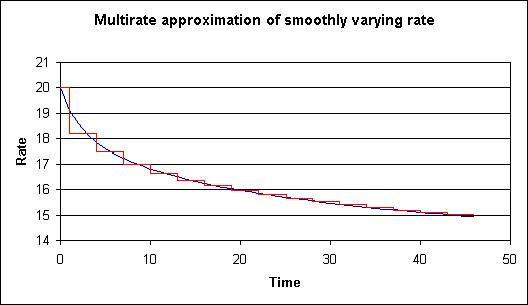
Superposition time is also required when multi-rate analyses are used to approximate situations in which the rate is slowly varying.
Superposition time is a time function that creates a common straight line when data from different rates are plotted on the same plot. The formulation of superposition time depends on the flow regime being analyzed. For example, superposition radial time is found by performing the superposition in time of the radial flow equation for each rate specified.
| Note: | The superposition time functions defined here and used in the software are different from those published in the literature. Superposition radial time is defined as the anti-log of that published in literature. Using this definition, data plotted on a semi-log plot of p vs. superposition radial time can be compared to a semi-log plot of p vs. Horner time. |
The following equations are the generalized forms of superposition time for each flow regime. They can handle any number of step changes in rate.
|
Superposition Time Functions |
|
|
Radial Time |
|
|
|
|
|
|
|
|
Spherical Time |
|
|
Pseudo-Steady State |
|


Superposition Time Example Calculations
| Note: | If there is a rate listed for when p = pi and time is zero, that rate is ignored in the calculations, and the rate corresponding to the first-time point is considered to be the rate at which the well has been flowing at up to that point. This is shown in the following set of calculations. |
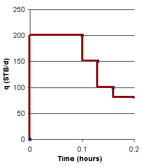
For a variable rate drawdown test, the following values are provided:
|
t (hrs) |
pwf (psia) |
q (stbbl / d) |
|
0 |
5000 |
0 |
|
0.10 |
4925 |
200 |
|
0.13 |
4920 |
150 |
|
0.16 |
4900 |
100 |
|
0.20 |
4890 |
80 |
Radial Flow Regime
The following procedure is used to calculate the superposition radial time at t = 0.2 hrs:
1. For the first rate, a well is flowing at 200 stbbl / d from the start of the test to the time point t = 0.2 hrs.

2. For the second rate, a well is flowing at –50 stbbl / d from t = 0.1 hrs to the time point t = 0.2 hrs.

3. The same is done for the remaining steps.


4. To get the superposition radial time, we add up all of the above times and take the anti-log of the result:

Linear Flow Regime
Using the same data set as above, calculate the superposition linear time at t = 0.2 hrs.
1. For the first rate, a well is flowing at 200 stbbl / d from the start of the test to the time point t = 0.2 hrs.

2. For the second rate, a well is flowing at –50 stbbl / d from t = 0.1 hrs to the time point t = 0.2 hours.

3. The same is done for the remaining steps.


4. To get the superposition linear time at t = 0.2 hrs, we add up all of the above times and take the square of the result:
