Editing Parameters Associated with the Analysis
When performing a decline analysis, you can create a best fit by editing the parameters associated with the analysis.
Traditional Decline Parameters
Parameters used in a traditional decline analysis are displayed in the Analysis Parameters pane.

Parameter descriptions are provided below:
| Parameter | Description |
|---|---|
|
Calc Method |
From this drop-down menu, you can select the method by which the decline analysis is calculated. (Options consisting of two parameters indicate the parameters to be calculated by Harmony.) ∆t | Qf — Decline rate (di), decline exponent (b), and abandonment rate (qf) are specified; forecast length (∆t) and EUR are calculated. ∆t | di — EUR, decline exponent (b) and abandonment rate (qf) are specified; forecast length (∆t) and decline rate (di) are calculated. ∆t | qf — Decline rate (di), decline exponent (b), and EUR are specified; forecast length (∆t) and abandonment rate (qf) are calculated. qf | Qf — Decline rate (di), decline exponent (b), and forecast length (∆t) are specified; abandonment rate (qf) and EUR are calculated. di | Qf — Forecast length (∆t), decline exponent (b), and abandonment rate (qf) are specified; decline rate (di) and EUR are calculated. di | qf — Forecast length (∆t), decline exponent (b), and EUR are specified; decline rate (di) and abandonment rate (qf) are calculated. di | b — Forecast length (∆t), EUR, and abandonment rate (qf) are specified; decline rate (di) and decline exponent (b) are calculated. Fixed Rate — A constant rate and forecast length are specified. dlim – dlim – qf | Qf — A terminal / limiting decline rate is added. This truncates a hyperbolic forecast at a set decline rate and the remainder of the forecast is exponential decline. Abandonment rate (qf) and EUR are calculated. dlim - Inclining Rate — The incline rate (negative decline rate) and end rate of an inclining line are specified. |
|
Start Date |
The end of production data and the date of the forecast start, represented by the middle point of the analysis line. |
|
qi |
The initial gas / oil production rate for the forecast. |
|
Qi |
The cumulative production at the start of the forecast. |
|
∆t |
The duration of the forecast. |
|
disec |
The effective secant decline rate at the start of the forecast. (Note: switch between di sec, di tan, and ai by pressing the decline rate type button) |
|
ditan |
The effective tangential decline rate at the start of the forecast.(Note: switch between di sec, di tan, and ai by pressing the decline rate type button) |
|
ai |
The instantaneous decline rate at the start of the forecast.(Note: switch between di sec, di tan, and ai by clicking the decline rate type button) |
|
b |
The decline exponent. This value is locked when using point selection for best fit. When selected, this value changes when you use point selection to create a best fit. |
|
qf |
The gas / oil production rate at the end of the forecast. |
|
End Date |
The date the forecast ends. |
|
∆Q |
The cumulative production that occurs during the forecast period. |
|
Qf |
The cumulative production at the end of the forecast — expected ultimate recovery (EUR). |
 t | Q
t | Q
Terminal / Limiting Decline Rate
The Terminal / Limiting Decline Rate begins as a hyperbolic decline curve and transitions into an exponential decline curve at a specified limiting effective decline rate, dlim. When the Terminal / Limiting Decline Rate option is selected in the Calc Method drop-down menu, a dlim value is required.
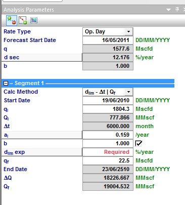
There are two options for the dlim value: “dlimexponential” and “dlimhyperbolic”. When you click 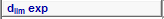 , it will toggle to
  ; clicking the option again will select "dlimexponential".
When using the “dlimexponential” option, the decline will transition such that the exponential portion of the decline will have an effective decline rate of the dlimvalue specified. When using the “dlimhyperbolic” option, the decline will transition when the hyperbolic portion reaches the specified dlim value. The exponential portion will then have an effective decline rate that is different from the dlim value.
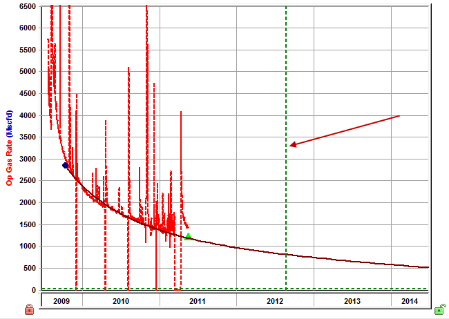
Note: The vertical dashed green line in the screenshot above indicates the transition from hyperbolic to exponential.
Terminal Decline Calculation Methods
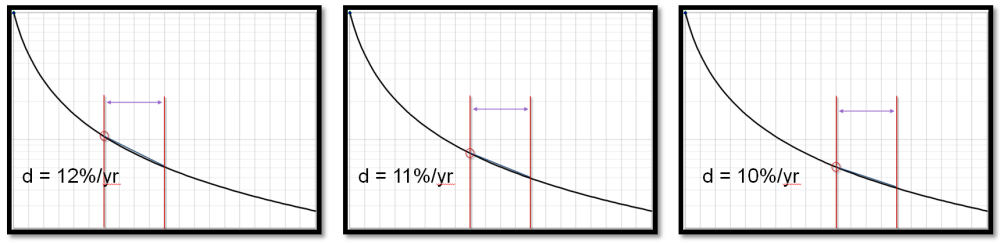
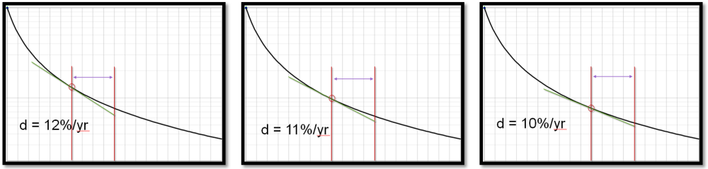
There are two ways to calculate the effective decline rate:
1. Secant
2. Tangent
All of the calculations go from your point of interest to a year ahead, but the difference is whether you are drawing a chord segment (secant line) or tangent line.
Note: The most common way to calculate the effective decline rate is by using the secant line, and because of this, references to the effective decline rate mean that the secant line is used.
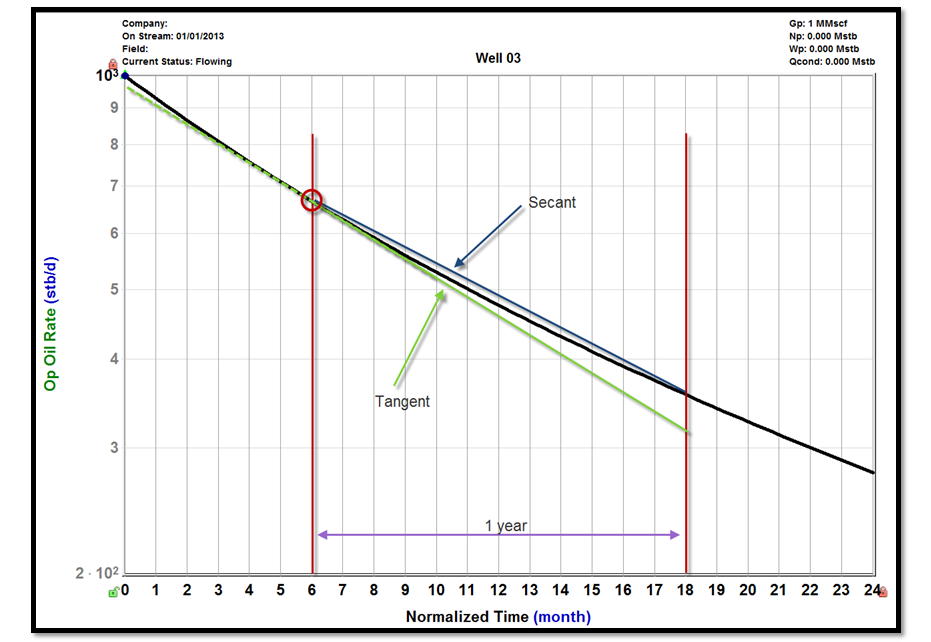
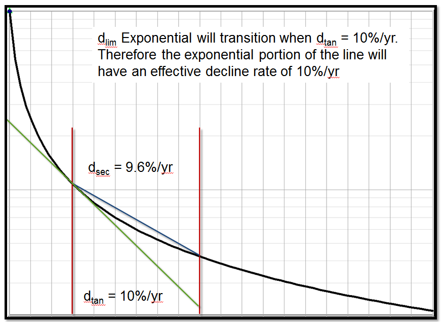
A dlim hyperbolic uses the secant line to calculate the effective decline rate. If you want a dlim hyperbolic of 10%, find where the 10% is calculated, and then switch from a hyperbolic decline to an exponential decline.
However, you cannot go from the hyperbolic to that chord segment line and expect a reasonable result. You need a smooth transition, so even though we used the chord segment to calculate the 10%, we need to use the tangent line to create the exponential section, which is not even 10%. This section is 10.4% for the remainder of the forecast.
![]()
The method described above used to be the default way of calculating terminal decline. Even though the secant / chord segment is how the effective decline rate is almost always calculated, when doing a dlim, we use the tangent line.
The transition from hyperbolic to exponential is smooth, with an exponential portion that is actually 10%. This is now the default way to calculate terminal decline.
Stretched Exponential Decline Parameters
Parameters used in a Stretched Exponential Decline analysis are displayed in the Analysis Parameters pane. Parameter descriptions are provided below:
| Parameter | Description |
|---|---|
|
Calc Method |
From this drop-down menu, you can select the method by which the decline analysis is calculated. |
|
Start Date |
The end of production data and the date of the forecast start, represented by the middle point of the analysis line. |
|
qi |
The initial gas/oil production rate for the forecast. |
|
Qi |
The cumulative production at the start of the forecast. |
|
∆t |
The duration of the forecast. |
|
qo |
Stretched exponential qo term. (The initial rate at the start of production. Not to be confused with qi, which is the initial rate at the start of the forecast.) |
|
n |
Stretched exponential n term. (Must be between 0 and 1.) |
|
t |
Stretched exponential t term. (Must be positive.) |
|
qf |
The gas/oil production rate at the end of the forecast. |
|
End Date |
The date the forecast ends. |
|
∆Q |
The cumulative production that occurs during the forecast period. |
|
Qf |
The cumulative production at the end of the forecast (EUR). |
|
EURg Infinite |
The EUR if the abandonment rate = 0. |
Multi-Segment Decline Parameters
Parameters used in a Multi-Segment Decline analysis are displayed in the Analysis Parameters pane, and are the same as the Traditional Decline parameters, with the following additions:
| Parameter | Description |
|---|---|
|
Defines whether the b value is entered, or referenced from a custom attribute |
|
|
|
Defines whether the |
|
|
Time constraint used to specify the transition point between segment 1 and 2 |
|
qmin |
Fluid rate constraint used to specify the transition point between segment 1 and 2 |
| (d sec)min | Decline rate constraint used to specify the transition point between segment 1 and 2 |

|
Cumulative fluid constraint used to specify the transition point between segment 1 and 2 |

 value is entered, or referenced from a custom attribute
Locking Initial Pressure in Material Balance
In a G MB analysis, you can lock the initial pressure while you manipulate the analysis line. This is done by selecting Yes from the Abd Calc drop-down menu for lock Pi.
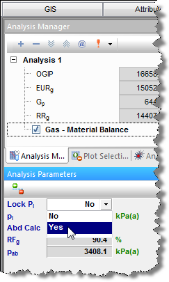
When the initial pressure is locked, the left point on the line turns gray and cannot be moved. (The initial pressure value can likewise no longer be edited.) The middle point on the line disappears, and the left point is now the pivot point.