Unconventional Reservoir Theory

Production Behaviour of Unconventional Reservoirs

The term 'unconventional' refers to production from very low-permeability formations. This often includes shale and very tight sands. When the permeability of a formation is very low, an enormous amount of surface area is required between the well completion and the reservoir to be able to produce at economic rates. This required area is achieved through multiple stages of massive fracture stimulations. The flow regime most often observed in these wells is linear flow. Linear flow may last several years and is often the only flow regime observed in the analysis. In addition to fractures created in the reservoir, linear flow can be caused by natural fracturing or enhancements to the natural fractures. For more information see Fracture Properties.

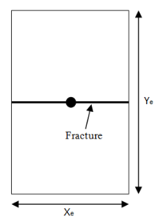
The effective drainage boundaries for these wells often coincide with the fracture length. In other words, drainage beyond the stimulated region is not significant and in the analysis method presented, this contribution is neglected. The base reservoir geometry used to develop this method is that of a single fracture centered in a rectangular reservoir, where the fracture width extends to the reservoir boundary. In this geometry, linear flow is observed until the reservoir width (Ye) boundary is reached, and the well enters boundary-dominated flow. The reservoir geometry is shown below:

Constant Flowing Pressure

Current analysis techniques in the industry use material balance time. Since material balance time is actually boundary-dominated flow superposition time, these analyses may appear to show boundary-dominated flow even when the reservoir is still exhibiting transient flow. In the method presented, no superposition functions are used, which avoids a bias towards any flow regimes. The production data is analyzed using a plot of reciprocal rate versus square-root time. In this plot, linear flow appears as a straight- line trend. The basic assumption is of infinite conductivity in the fracture; finite conductivity manifests as a positive intercept on the plot. The equations presented are based on the assumption of a constant flowing pressure at the well. This is a reasonable simplification for tight gas and shale production, in which wells are typically produced under high drawdown.

Based on the straight-line behaviour of the square root time plot, the simplest form of the linear flow equation is:

Equation 1

In this equation, the intercept captures a number of near well effects, such as skin and finite fracture conductivity, and the slope is given by:

For oil:

Equation 2a

For gas:

Equation 2b

From the slope of the equation, fracture half-length and permeability are determined as a single product. To determine either explicitly, the other parameter must be known.

To determine the skin effect, the intercept of the line is used with the following:

For oil:

Equation 2c

Equation 2d

For gas:

Equation 2e

Equation 2f

Duration of Linear Flow

When a well is producing under constant flowing pressure, the distance of investigation can be obtained from the following equation during the linear flow period:

Equation 3

Combining this equation with the reservoir geometry detailed in the diagram presented previously, the end of linear flow is given by the following:

Equation 4

Equation 4 can be rearranged as follows:

Equation 5

This is not a practical form of the equation, since permeability (k) and reservoir width (Ye) are usually not explicitly known. The permeability is tied into the (xf√k) term and reservoir width is related to the drainage area (A); however, both of these are related to fracture half-length (xf). Using the definition of drainage area (A = 2 * xf * Ye), equation 5 becomes:

Equation 6a

The (xf√k) term is determined from the slope of the square-root time plot using a rearranged form of equation 2. For unconventional gas reservoirs, xf√k departs from its analytical value as the pressure drawdown, DD, becomes higher. To correct for this drawdown effect, a correction factor, fcp, is implemented in the gas constant pressure module, which allows for a more accurate determination of xf√k.

DD and fcp are defined as follows:

Equation 6b

Equation 6c

xf√k can be determined by using following equations:

For oil:

Equation 7a

For gas:

Equation 7b

Substituting equation 7 into equation 6a, the duration of linear flow (and hence the beginning of boundary-dominated flow) is determined using the following equation:

For oil:

Equation 8a

For gas:

Equation 8b

An approximation of the gas equation can be obtained by replacing pseudo-pressure terms with:

Equation 8c

and cti by the inverse of pi

The major unknown in determining the end of linear flow is the effective drainage area. Analog wells can be used to determine an appropriate range of drainage areas for the subject well. Well spacing can provide an upper bound on drainage area in high-density developments. Interpretation of flowing material balance can be used to determine a minimum area based on the current production data.

Boundary-Dominated Flow

Given the geometry of the reservoir considered, linear flow is followed directly by boundary-dominated flow. There are two ways to represent this flow regime for purposes of forecasting: (a) pseudo-steady state equations, material balance time, and pseudo-time; (b) traditional (Arps) hyperbolic decline. In the interest of keeping the method simple and practical, the hyperbolic decline method is used. Hyperbolic decline is defined in the following equation:

Equation 9

In this equation, qi and ai are flow rate and decline rate (respectively) at the start of the forecast period; and t is the time that has elapsed since the start of the forecast. Since the hyperbolic decline forecast starts at the end of linear flow, the flow rate, decline rate, and time will be with respect to time at the end of linear flow (telf). The decline exponent (b) is selected to be between 0 and 0.5, which are typical values for boundary-dominated flow in gas. Equation 9 is then rewritten to represent this:

Equation 10

Equation 1 is rewritten to show how rate at the end of linear flow (qelf) is determined based on the interpretation of the square-root time plot:

Equation 11

Decline rate from the hyperbolic decline equation is defined as:

Equation 12

In order to determine decline rate at the end of linear flow (aelf), an expression is needed for decline rate during linear flow. This is obtained by combining Equation 1 and Equation 12:

Equation 13

This equation is now written to reflect the decline rate at the end of linear flow:

Equation 14

From Equation 14, it is also apparent that if b is negligible, the equation reduces to:

Equation 15

Once a decline exponent (b) is selected, Equation 10 can be used for any duration of forecast, and even to determine the production forecast based on an abandonment rate.

Variable Flowing Pressure

In the initial development of this interpretation technique, constant flowing pressure has been assumed. An additional case for variable flowing pressure may also be considered when interpreting the square-root time plot. The standard y-axis of reciprocal rate is simply replaced with normalized pressure to account for changes in flowing pressure during the linear flow portion of the data. Transient linear flow appears to be a straight line in the normalized pressure versus square-root of time plot. The slope of the straight line, m, is used to calculate xf√k with the following:

For oil:

Equation 16a

For gas:

Equation 16b

As stated earlier, the observation has been that most unconventional wells are produced at very high drawdown rates to maximize recovery. Because of this common practice, the forecasting approach in the variable pressure module uses hyperbolic decline with the assumption of constant pressure for the duration of the forecast.

Superposition Time

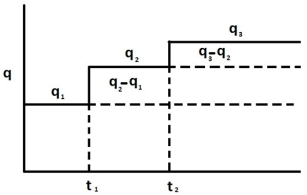
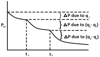
Superposition is a mathematical tool. You can use simple solutions (such as constant rates) to produce complex ones (such as variable rates). Superposition uses the theory that a rate that changes from q1 at time t to a new rate q2 is equivalent to q1 continuing forever, superposed, or added on (q2 - q1) starting at time t and continuing forever.

For unconventional reservoirs, two superposition time functions are commonly used in production analysis: linear superposition time and material balance time.

Linear superposition time is given by:

Equation 17a

Material balance time is given by:

Equation 17b

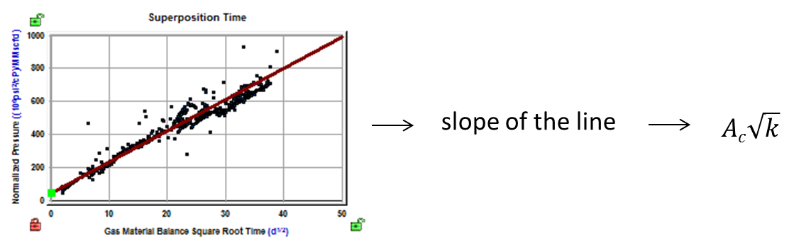
Both two superposition time functions can effectively convert variable rates to their equivalent constant rates solutions. Therefore, the plot of versus linear superposition time (or square root of material balance time) on a Cartesian graph results in a straight line. The slope of this line (m’) can be used to calculate :

For oil:

Equation 17c

For gas:

Equation 17d

Using Pseudo-Time

The above derivations used for the Unconventional Reservoir Model (URM) analysis do not account for variation in total compressibility. It is possible to account for variation in total compressibility and fluid viscosity by using pseudo-time.

Pseudo-time is defined as follows:

For oil:

For gas:

In these equations, , is average pressure over the volume investigated at a given time t.

Note:   The correction factor, f_CP, (defined in Equation 6c) is another way to account for variation in gas compressibility. Therefore, when pseudo-time is used, there is no need to use the correction factor, f_CP, in calculations.

Accounting for Variation in Rock and Fluid Properties in the Oil URM

In the descriptions above, URM analysis for gas is done in terms of pseudo-pressure, and URM analysis for oil is done in terms of pressure. This is done because for the oil case, a variation of oil properties (such as viscosity, compressibility, and the formation volume factor) is considered to be negligible, and formation compressibility and permeability are assumed to be constant (no geomechanical effects).

However in some cases, it is important to account for a variation in oil and formation properties. This can be done similarly to how it is done for gas cases, by introducing oil pseudo-pressure:

When the oil URM calculation is modified to use pseudo-pressure, the FMB plot within the URM dashboard is also modified. For information on modifications for the oil FMB plot, see Accounting for Variation in Oil Properties (FMB).

Note:   This approach is used and described in literature, including Behmanesh et al. (2015), Stalgorova and Mattar (2016).

Accounting for Changing Oil Saturation in the Oil URM (theory)

The oil URM analysis assumes single-phase (oil) flow in the reservoir. However in reality, pressure often drops below the bubble point, which results in two-phase flow (oil and liberated gas). Additional modifications have to be done to account for such cases.

If we consider the flow of the oil phase in the reservoir, there are two qualitative changes that occur when the pressure drops below the bubble point:

• A large increase in total compressibility of the system (due to gas liberation)
• A decrease in the effective oil permeability (due to relative permeability)

Accounting for a large increase in total compressibility

Using pseudo-pressure and pseudo-time already accounts for the variation of total compressibility with pressure. Therefore, no additional modifications are required for two-phase flow.

However, it is important to keep in mind that the pseudo-time transformation is inexact, which makes the results inaccurate for certain cases. This inaccuracy is larger when the variation in total compressibility is larger. Therefore, we expect the inaccuracies due to the use of pseudo-time for two-phase flow to be larger, than for single-phase (oil) flow.

Accounting for relative permeability

Modifications were suggested for the definition of pseudo-pressure to account for relative permeability by Raghavan (1976), and modifications were made for various cases later on (e.g., see Behmanesh et al. (2015) for modifications in linear flow analysis). Since pseudo-pressure and pseudo-time transformations already account for the change of permeability with pressure, they can be easily adapted to include the relative permeability term as well.

Two-phase oil pseudo-pressure is defined as:

Two-phase pseudo-time is defined as:

where k_ro is the relative permeability of oil in the two-phase (oil and gas) system.

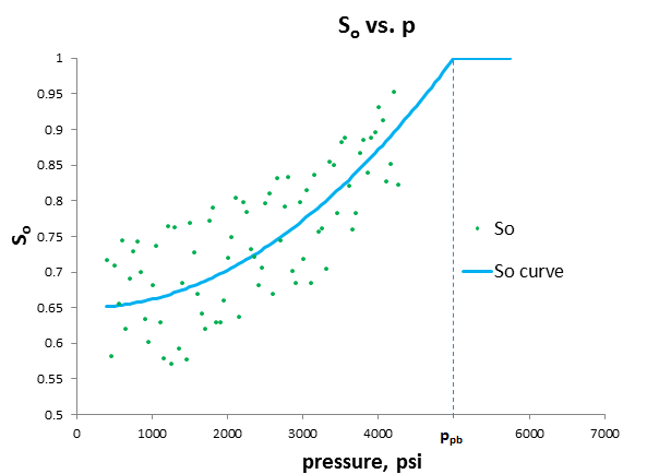
Both these definitions include the k_ro (S_o (p)) term. k_ro (S_o) is a known dependency (given by relatively permeability curves). However, S_o (p) is an unknown function and it may vary depending on the way the well is produced. To address this issue, Raghavan (1976) assumed that the producing gas-oil ratio (GOR) can be estimated as:

This can be re-arranged as:

This approximation can be used to generate the relationship S_o (p) between S_o and p_wf as described below. For each production data point:

1. Calculate the right-side of the equation above (use producing GOR; evaluate R_s, µ_o, B_o, μ_g, and B_g at p_wf). This gives the relationship between k_rg / k_ro and p_wf.

2. Using relative permeability curves, generate the relationship between k_rg / k_ro and S_o.

3. Use the relationship between k_rg / k_ro and p_wf, and the relationship between k_rg / k_ro and S_o to estimate S_o for each production data point.

4. Plot S_o vs. p_wf.

5. Approximate the obtained scatter by a smooth curve. Use the S_o (p) relationship defined by the curve to calculate two-phase pseudo-pressure and pseudo-time.

Application to Horizontal Wells

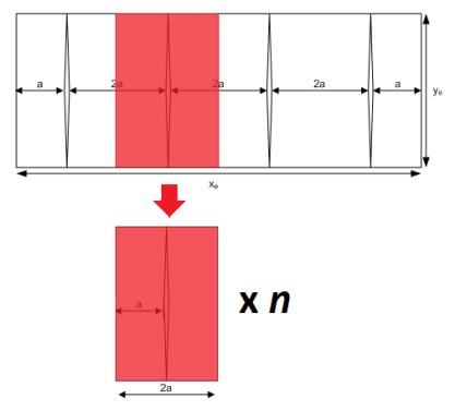
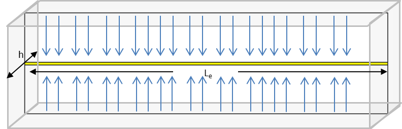
The majority of wells in unconventional gas production are horizontal wells with multiple stage fracturing. The approach first considered with the development of this method is to treat the horizontal wellbore as a fracture, and incorporate fracture stimulation in this well as part of the effective permeability interpreted on the square-root time plot. An additional method has been incorporated using the same process as that developed for a single fracture. If the horizontal well is cased, or contributes very little production compared to the fractures, the well can be treated as a series of fractures in the reservoir. In a well with n equally spaced and identically sized fractures, the single fracture model can be multiplied by n fractures to represent the whole well. The linear flow into the fractures is followed by boundary-dominated flow when no-flow boundaries are formed between adjacent fractures. This layout is displayed below with its relationship to the single-fracture model.

Applying this Theory to IHS RTA

This theory applies to using production data to identify the linear flow parameter and interpret the linear flow parameter for different completion types.

Using Production Data to Identify the Linear Flow Parameter

Equations 16a and 16b can be rewritten as:

For oil:

Equation 18a

For gas:

Equation 18b

Note:   Equations 17c and 17d can be rewritten in a similar way.

These equations are derived for the case where the well is being produced through a single fracture. For this case, the total area to flow (Ac) can be calculated as:

Equation 19

Therefore, equations 20a and 20b can be rewritten in a general form:

For oil:

Equation 20a

For gas:

Equation 20b

Where A_c is total area to flow.

In equations 20a and 20b, the right-side of the equation is known: m, and is defined by production data (the slope of the line for normalized pressure plotted against a function ), and the remaining parameters are known for reservoir and fluid properties. Therefore, we can calculate the linear flow parameter using the top-left plot on the unconventional reservoir model (URM) dashboard.

Note:   A_c represents the total area to flow, without any assumptions whether the well is producing through a single fracture, through multiple fractures, or through a non-fractured horizontal wellbore.

Interpreting the Linear Flow Parameter for Different Completion Types

Once the value for the linear flow parameter is calculated, it can be interpreted differently depending on the type of completion. With URM analysis, three types of completion are selectable from the Model Type drop-down list.

The following sections describe how the linear flow parameter is interpreted for each model type.

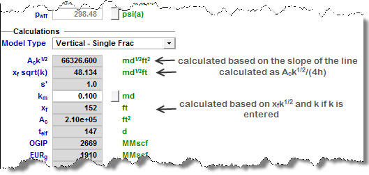
Vertical - Single Frac Model Type

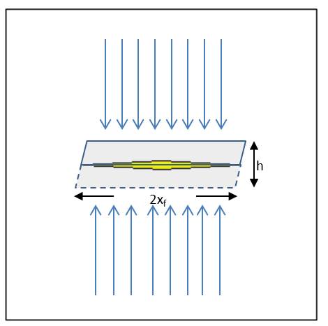
In this case, it is assumed that the well is being produced through a single fracture. We can observe linear flow towards the fracture from both sides. The total area to flow (Ac) can be calculated as:

Equation 21

Where h is the known net pay. Once is calculated, is also calculated and reported.

If you enter the value for permeability, x_f will be calculated based on the known value of permeability, and the previously calculated .

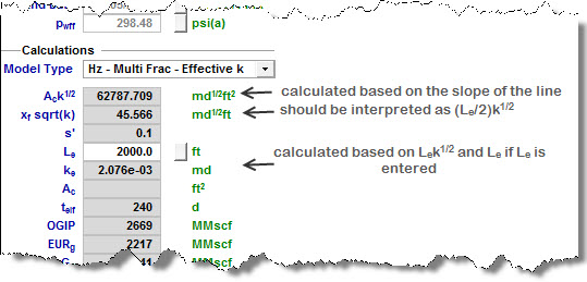
Horizontal Multifrac - Effective k Model Type

In this case, it is assumed that the well is being produced through a horizontal wellbore without fractures. This model can also be used when the well is fractured, but we do not model each individual fracture; instead we account for all the fractures by using higher effective permeability. Then, we can observe linear flow towards the wellbore.

Total area to flow (Ac) can be calculated as:

Equation 22

Where h is the known net pay. Once is calculated, can also be calculated.

Note:   As there is no x_f in this model type, the parameter should be interpreted as .

If you enter the value for effective horizontal wellbore length, L_e, effective permeability k_e will be calculated based on the known L_e and the previously calculated .

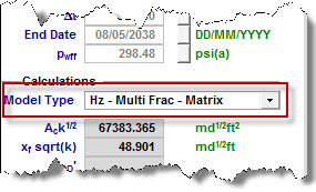
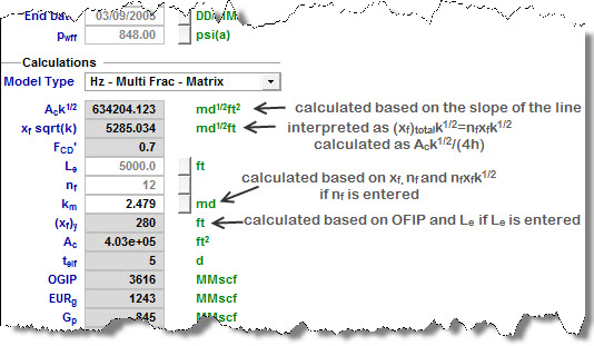
Horizontal Multifrac - Matrix Model Type

In this case, it is assumed that the well is being produced through multiple fractures (n_f = number of fractures). Then, we can observe linear flow towards each fracture.

The total area to flow (Ac) can be calculated as:

Equation 23

Where h is the known net pay. Once is calculated, can also be calculated.

For this completion type, there is another relationship between model parameters:

Equation 24

Where:

OFIP: original fluid in place – this value can be obtained from the Flowing Material Balance plot

h: net pay; known reservoir property

φ: porosity; known reservoir property

S_fi: initial saturation of the modeled fluid (oil or gas); known reservoir property

B_fi: initial formation volume factor of the modeled fluid (oil or gas); known fluid property

L_e: effective horizontal well length

x_f: fracture half-length

In Equation 24, all parameters except for L_e and x_f are known. Therefore, if you enter the value for L_e, x_f can be calculated.

If you enter the value for n_f, permeability can be calculated based on the previously calculated , x_f, and the given n_f.

Most Likely Model

This model is a new methodology for identifying the possible range of stimulated reservoir volume (SRV) configurations based on specified well performance data, assumed system geometry, and known external system constraints.

The method is based on providing single values for known completion and petrophysical properties, and lower / upper limits for unknown parameters. The method is suitable for early well performance data, where transient linear flow is dominant.

The method is graphics-based with a plot of the exposed area of the fractures (Ax) versus drainage area of the reservoir (Ad). Based on user-defined constraints and limits, this plot defines a region that contains the full set of possible SRV configurations.

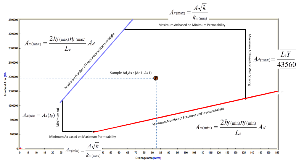
The definition of the allowable range of Ax versus Ad is identified in two parts.

Part 1: Identify the Region that Defines Minimum and Maximum Values for Ax and Ad

Limiting values for Ax are determined as follows:

Important:   All of the equations below are referenced earlier in this topic.

Equation 18a

Equation 18b

Where A√k is extracted from the slope of the square root straight line on the specialized plot, and km(min) and km(max) define the acceptable range of the unknown parameter, Stimulated Region Permeability.

The parameter km is considered to be an effective permeability, inclusive of any natural or induced fractures that have been activated (or are naturally active) and are connected to the primary hydraulic fracture network, but it does not include the primary fracture permeability. In other words, it is the permeability that acts directly on the primary hydraulic fracture system. Ax is defined as the total matrix area exposed to fractures. For a fracture of half-length (xf), Ax is defined as:

Equation 18c

Limiting values for Ad are determined as follows:

Equation 18d

Equation 18e

Where:

Ad(tp) equals the currently contacted drainage area, which is determined from a combined analysis of the square root straight line and the flowing material balance (Anderson et al. 2010).

Y equals the projected average distance between adjacent laterals once the field has been fully developed.

Based on the above, a box-shaped region can be defined on a plot of Ax versus Ad.

Part 2: Identify the Functional Relationship between Ax and Ad

Assuming parallel transverse fractures (slab model) of uniform distribution and length, Ad is a linear function of Ax as follows:

Equation 19a

If the fracture network is assumed to be 2-dimensional (matchstick geometry), the coefficient in the above equation becomes 4. If the fracture network is assumed to be 3-dimensional (sugar cube geometry), the coefficient becomes 6.

Since hf and nf are unknowns, we can define the minimum and maximum functional relationship between Ax and Ad, assuming that we can provide allowable ranges for hf and nf.

Equation 19b

Equation 19c

The above equations plot as straight lines through the origin on the Ax versus Ad plot. The intersection of the previously defined rectangular region with these straight lines yields a region that contains all the possible Ad and Ax combinations.

Formulae for calculating reservoir / completion properties, given a sample configuration (Ad1, Ax1) from the Ax - Ad region, are shown as follows:

Equation 19d

Equation 19e

Equation 19f

Equation 19g

The mass center of the Allowable Ax versus Ad region is used to calculate the Most Likely values.