Creating an Unconventional Reservoir Analysis

To create an unconventional reservoir analysis:

1. Launch an entity for analysis.

2. Click the Unconventional Reservoir thumbnail; then select the type of worksheet you want to create.

• Deterministic — creates an analysis based on known parameters.
• Most Likely — creates an analysis based on a range of values. Produces "most likely" values that can be used to generate a deterministic model.

3. Best fit the analysis to the data by doing one of the following:

• selecting data points
• manipulating the analysis straight line

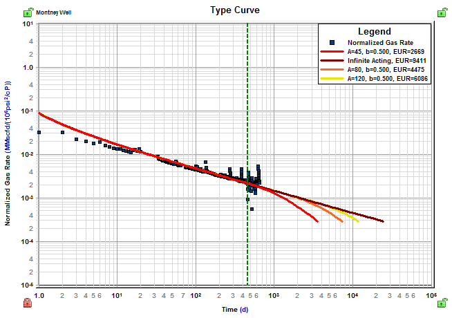
The typecurve and forecast plots display the generated production forecasts, but also include the historical trend. This can be used as a validation of the interpretations. In addition, a green vertical line shows where linear flows end, and boundary-dominated flow begins. If only linear flow has been observed (the data does not deviate from the slope on the square-root time plot), this line should be displayed at the end of the data, and the flowing material balance (FMB) interpretation would be considered a minimum OOIP / OGIP.

It is also possible to display the Raw Data Derivative and the Beta-Derivative options for the data on this plot by clicking the corresponding boxes under Typecurve Options in the Unconventional Reservoir pane.

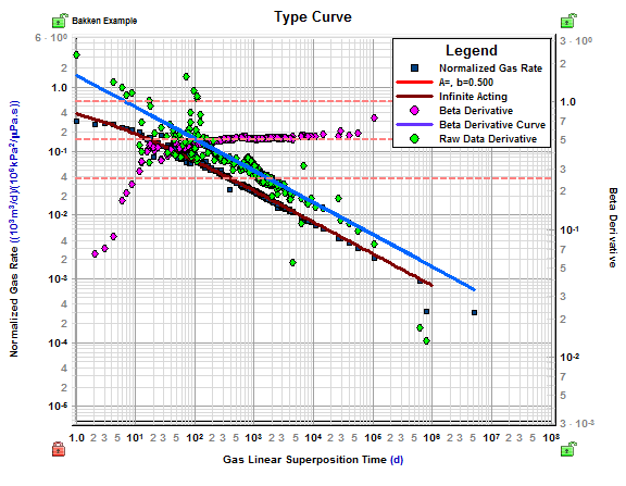
In addition to the forecast based on the OOIP / OGIP interpreted from the FMB (bright red forecast line), an infinite-acting case of continuing linear flow is also created (brown forecast line) to provide an upper limit forecast. Often this forecast will appear to truncate before the abandonment rate is reached. If the abandonment rate has not been reached, all forecasts are truncated at a duration of 100 years.

In the case that boundary-dominated flow has not been observed, additional scenarios with larger drainage areas can be created by clicking the User Type Curves icon () in the typecurve or forecast toolbar. This icon launches a table for up to five additional areas to be entered.

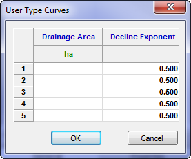
For each area, a separate decline exponent may also be used. Each additional area is displayed on the typecurve and forecast plots, with the respective EUR values listed in the legend.