Advanced Analytical Models Tab

Subtopics:

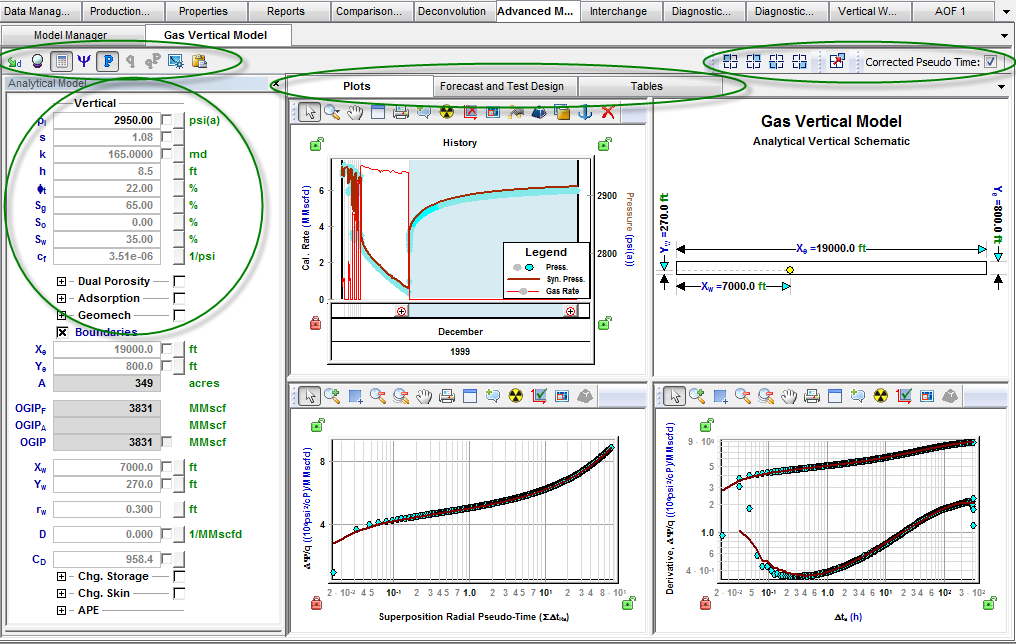
Toolbar

The left-side toolbar is located just below the analytical model tab and provides the following options (described from left-to-right):

Apply Defaults — Populates all parameters with available defaults. In WellTest, default values are available from analyses, legacy models, and advanced models.
Automatic Parameter Estimation — Starts automatic parameter estimation.
AutoCalc — When selected, the model calculates immediately following a change to the model's input parameters. When deselected, the model only recalculates when you click the Synthesize icon.
Synthesize — Calculates the model.
CalcP — Calculates a synthetic pressure using measured rate as an input.
CalcR — Calculates a synthetic rate using measured pressure as an input.
CalcBoth — Calculates a synthetic pressure using measured rate as the input, and calculates a synthetic rate using measured pressure as an input.
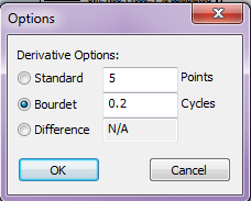
Derivative Options — Launches a dialog box where you can specify derivative calculation options.

Copy to / Paste from Clipboard -- "Copy to Clipboard" copies the current values of model parameters to the clipboard. "Paste from Clipboard" pastes the model parameters that have been copied to the clipboard. If model parameters have not been copied to the clipboard, the Paste from Clipboard option is not available.

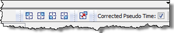
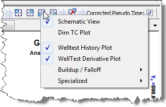
Another toolbar is located on the far right. With the first four icons, you can replace one of the existing plots with a different plot, and with the fifth icon, you can add a new floating view. When any of these icon are clicked, a menu with available plot types is displayed. There is also a checkbox for Corrected Pseudo Time.

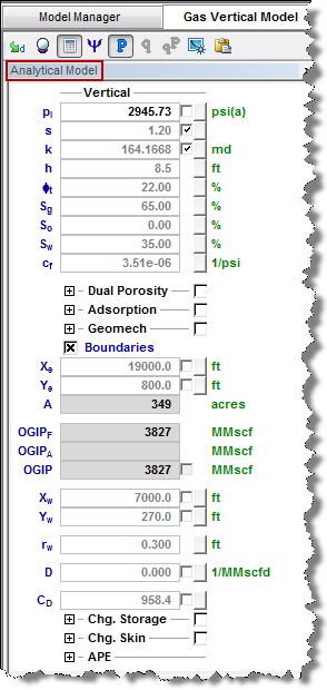
Analytical Model Inputs Pane

The Analytical Model Inputs pane is where all modeling parameters are entered. The available model parameters depend on the model type and fluid type, which were selected in the Model Manager when creating the advanced analytical model.

Plots Tab

This view is split into four sections, each displaying a schematic or a plot. The item displayed in each section can be changed using the icons on the right-side toolbar.

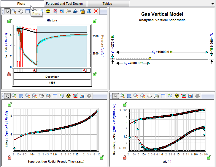
The Schematic is an overhead view of the reservoir with dimensions for size and well location. Dimensions and well location can be adjusted by clicking-and-dragging over any of the light blue arrows.
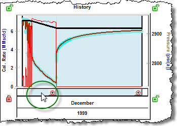
The History plot is a Cartesian plot of the measured and synthetic data. It is used to select the flow and shut-in periods that are displayed on the Specialized and Derivative plots. Click the bottom section of the plot to select or deselect a region. Multiple flow and shut-in periods may be selected at the same time.

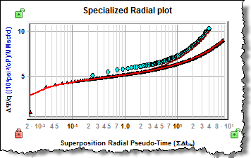
Specialized plots are designed to display the data from both drawdown (or injection) and buildup (or falloff) flow periods on the same plot. They linearize the data for a specific flow regime. Specialized plots for different flow regimes are available from the Plot Selection icon on the right-side toolbar.

The Derivative plot shows the data and the Der (semilog derivative) for all periods selected on the History plot.
The Buildup / Falloff plots are the traditional plots used to linearize the data for a specific flow regime. They only display data from shut-in periods.

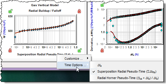
As shown above, time options my be changed by right-clicking the x-axis title of Specialized, Buildup / Falloff, or Derivative plots.

Forecast and Test Design Tab

In the Forecast and Test Design tab, you can estimate reservoir gas, oil, or water production rates / pressures using a model based on your specified reservoir properties and forecasting parameters.

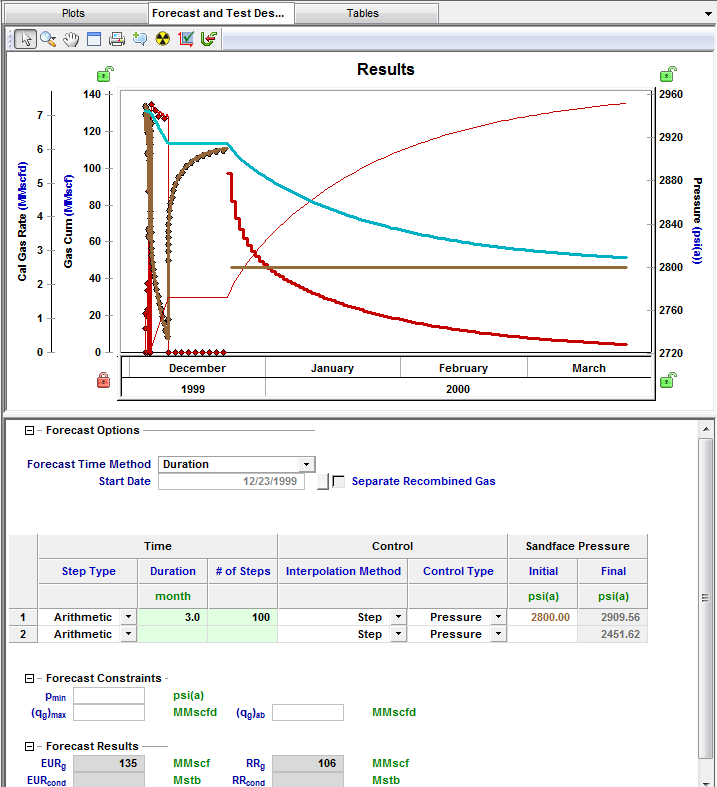
This tab has two sections: a Results plot and a Forecast table.

Note:

Production / pressure history is not required to generate test design scenarios. The parameters of the test design scenario are entered in the Forecast table.

Results Plot

The Results plot shows the production history, pressure data, and the model match, if they exist. In addition, forecasted data is displayed, which consists of a fluid rate, forecasted pressure, and the average reservoir pressure. If more than one forecast case is present, the results of each are displayed on the Results plot.

Forecasting

Forecasting in the Advanced Models takes the production history into account and does not commence assuming static reservoir conditions. A forecast may be generated based on your reservoir model parameters and specified forecasting parameters.

See Forecasting in Advanced Models for details.

Forecast Parameters

Several additional features exist in the Forecast pane that can be used to customize the forecast. This pane consists of the following three sections:

1. Forecast Options

2. Forecast Constraints

3. Forecast Results

Note:

Each of these sections can be expanded or collapsed by clicking the +/- box.

Forecast Options

The Forecast Options section is where forecast periods are defined according to either durations (e.g., months), or dates.

Setting the forecast time method to Duration begins a forecast at a specified start date. Forecast periods are then defined in the forecast table according to a length of time (the default is months). For each forecast period, different operating conditions can be specified.
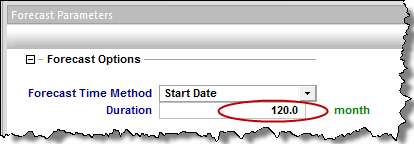
Setting the forecast time method to Start Date creates a forecast of a specified length of time (the default is months). Forecast periods are then defined in the forecast table according to calendar dates.

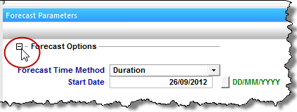
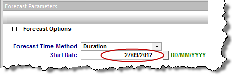
If you select Duration from the Forecast Time Method drop-down menu, the Start Date is automatically populated. (You can change this date later, if needed.)

If you select Start Date from the Forecast Time Method drop-down menu, enter a value for Duration (i.e., the total length of the forecast).

The Forecast Flowing Pressure can also be set in the Forecast Options section. If a Gas Condensate well is being analyzed, the Separate Recombined Gas option is available in Forecast Options.

Further details about each forecast period are entered in the forecast options table.

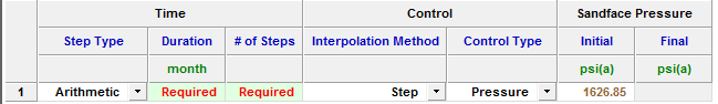
Each row of the table above represents a forecast period. An additional forecast period can be added each time an operational change is encountered (e.g., the flowing pressure decreases when a compressor is added). The forecast options table has the following sections:

Time – defines the length of each forecast period and each timestep, and has the following columns:

Step Type – sets the spacing of the timesteps, and can be set to either Arithmetic or Logarithmic. The Arithmetic step type spaces the number of timesteps equally over the total duration of the period, whereas the Logarithmic step type spaces the number of timesteps logarithmically (i.e., increased density near the beginning of the forecast).

Forecast Time Method (Duration / Start Date) – sets the length of the forecast period. If Forecast Time Method is set to Duration, this column displays Duration. If Forecast Time Method is set to Start Date, this column displays Start Date.

# of Steps – sets the number of timesteps in the forecast period.

Control – defines how the operating conditions change over the forecast period, and has the following columns:

Interpolation – can be set to either Step or Ramp. Step keeps the control type constant over the forecast period. Ramp varies the control type linearly from an initial value, to a final value.

Control Type – sets what is used to calculate the forecast. The options for this column are dependent on the type of analysis being performed. For analytical models and typecurves, choices are pressure, and the primary fluid of the analysis. For example, when creating a Gas Analytical Model, the forecast can be run using either flowing pressure, or gas rate. For numerical models, choices are pressure, and any fluid that is present in the model.

Sandface Pressure – If the Control Type is set to Pressure, this column is displayed, and it is used to set the flowing pressure for the forecast period. If Interpolation is set to Step, only the initial pressure cell is editable. If Interpolation is set to Ramp, initial pressure and final pressure are selectable.
Gas/Oil/Water Rate – If the Control Type is set to Gas, Oil, or Water, this column is displayed, and it is used to set the rate for the forecast period. If Interpolation is set to Step, only the initial rate's cell is editable. If Interpolation is set to Ramp, initial rate and final rate are editable.
Ratios – If a gas condensate system is being forecasted, this column is displayed, and it is used to define how relevant ratios change over the forecast (e.g., CGR, WGR, WOR, GOR). A separate interpolation method can be set for the ratios. This interpolation method applies to all ratios, but it is independent of the interpolation method set for the control.

Forecast Constraints

The Forecast Constraints section is where maximum rate conditions and abandonment rate conditions for the forecast can be entered. Available constraints depend on the analysis type, and could include the following:

p_min – The minimum allowable sandface flowing pressure during the forecast. In order to ensure flowing pressure does not go below this value, rates are adjusted.
(q_g)_max – Sets a maximum gas rate during the forecast. In order to maintain the maximum gas rate constraint, flowing pressure is adjusted.
(q_w)_max – Sets a maximum water rate during the forecast. In order to maintain the maximum water rate constraint, flowing pressure is adjusted.
(q_o)_max – Sets a maximum oil rate during the forecast. In order to maintain the maximum oil rate constraint, flowing pressure is adjusted.
(q_g)_ab – Sets the abandonment gas rate for the forecast. When the abandonment rate is reached, the forecast ends.
(q_w)_ab – Sets the abandonment water rate for the forecast. When the abandonment rate is reached, the forecast ends.
(q_o)_ab – Sets the abandonment oil rate for the forecast. When the abandonment rate is reached, the forecast ends.

For analytical models, the available constraints include a minimum flowing pressure, as well as maximum and abandonment rates corresponding to the fluid being analyzed. For example, a gas analytical model includes p_min, (q_g)_max, and (q_g)_ab. Numerical models include minimum flowing pressure, as well as maximum and abandonment rates for all fluids in the model.

Forecast Results

The Forecast Results section is where the results of the forecast are summarized. Available results depend on the analysis type, and could include the following:

EUR – Expected Ultimate Recovery (EUR).

RR – Remaining Recoverable (RR).

Note:

For wells with historical data, EUR is defined as the cumulative of the historical data up to the beginning of the forecast, after which time, the synthetic cumulative calculated from the model is used until the end of the forecast.

For typecurve and analytical models, EUR and RR of the fluid being analyzed are available. When analyzing a gas condensate system, EUR and RR of the condensate phase are also available. For numerical models, EUR and RR of all the fluids in the model are available.

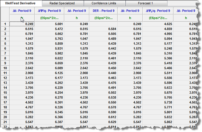
Tables Tab

The Tables tab is a tabular display of the data within each plot in the Plots tab.